Using the penalty function method, the solution of nonlinear programming problems can be transformed into solving a series of unconstrained extremum problems. This method is also referred to as the Sequential Unconstrained Minimization Technique, abbreviated as SUMT. The idea behind the penalty function method for solving nonlinear programming problems is to construct an augmented objective function with parameters by appropriately defining penalty functions based on the constraint functions of the problem, thus converting the problem into an unconstrained nonlinear programming problem. There are mainly two forms: one is called the external penalty function method, and the other is called the internal penalty function method.
11.3.1 External Penalty Function Method
For a general nonlinear programming problem:
min f(X)

Let

Thus, (1) is transformed into an unconstrained optimization problem:

If we set

Then it is transformed into solving the following optimization problem:

Where T(X, M) is called the penalty function, M is the penalty factor, and the term with M is called the penalty term. The penalty function only punishes points that do not satisfy the constraints: when X ∈ D (D is the feasible region), satisfying each gi(X) ≥ 0, hi(X) = 0, thus the penalty term = 0, and no punishment is applied. When X is outside D, there must be constraints where gi(X) < 0 or hi(X) ≠ 0, hence the penalty term > 0, and punishment is applied.
The iterative steps of the SUTM external point method (penalty function method) are as follows:
(1) Arbitrarily set an initial point X0, take M1 > 1, set the allowable error ε > 0, and let k = 1;
(2) Solve the unconstrained extremum problem

for the optimal solution, denoted as Xk = X(Mk), that is

(3) If Mp(Xk) > ε, then take Mk > M (Mk+1 = αM, α = 10), let k = k + 1 and return to (2), otherwise, stop the iteration. The optimal solution is X* ≈ Xk.
The disadvantage of the penalty function method is that each approximate optimal solution Xk is often not a feasible solution, but only approximately satisfies the constraints, which may not be usable in practical problems; the computational load in solving a series of unconstrained problems is too large, especially as Mk increases, which may lead to errors.
Example 11.3.1 Solve the following nonlinear programming model:


Solution: First, establish the penalty term function li11_3_1p.m file as follows:

Then establish the penalty function li11_3_1t.m file as follows:

Finally, establish the main function li11_3_1.m file as follows:
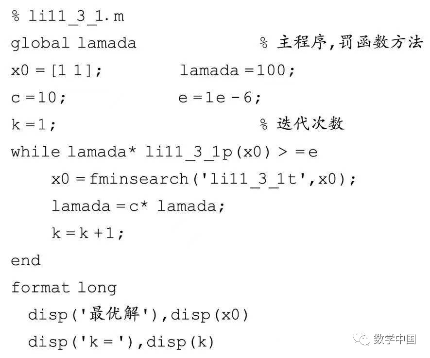
Executing li11_3_1.m yields

11.3.2 Internal Penalty Function Method
Consider the problem:

Let the set D0 = {X | gi(X) > 0, i = 1, 2, …, m} ≠ φ, where D0 is the set of all strictly interior points in the feasible region. Construct the barrier function:

Let

or

Then rb(x) is called the barrier term, and r is the barrier factor. Thus, problem (2) is transformed into solving a series of extremum problems:

The iterative steps of the interior point method are as follows:
(1) Given an allowable error ε > 0, take r1 > 0, 0 < β < 1;
(2) Find an interior point X0 ∈ D0 of the constraint set D, let k = 1;
(3) Using Xk-1 ∈ D0 as the initial point, solve

where X ∈ D0 is the optimal solution, denoted as Xk = X(rk) ∈ D0;
(4) Check if |rkb(Xk)| ≤ ε, if satisfied, stop the iteration, X* ≈ Xk; otherwise, take rk+1 = βrk, let k = k + 1, and return to (3).
Example 11.3.2 Use the interior point method to solve the following linear programming problem:

Solution: First, write the li11_3_2.m program code as follows:
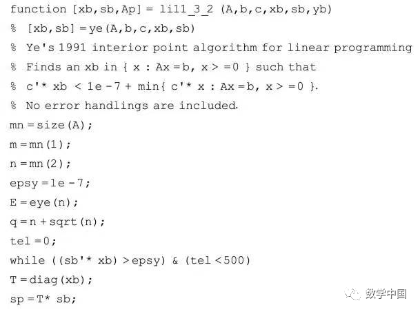
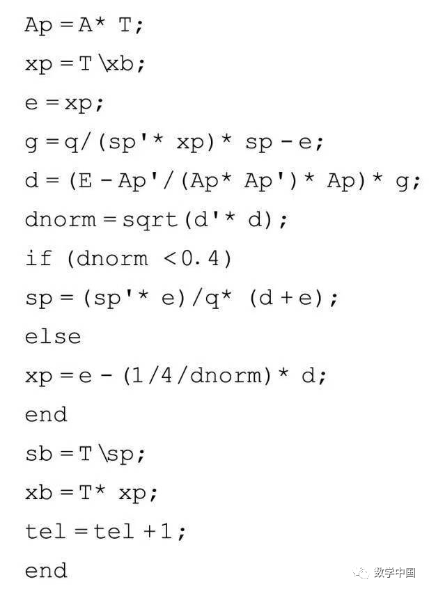
Next, write the li11_3_2zhu.m program as follows:
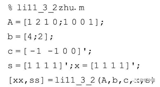
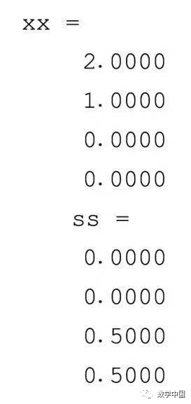
The program execution result is:
