The classic emergent “glider” in the Game of Life
The Game of Life by Coway was introduced in a previous article, which is a cellular automaton model. It considers a plane resembling a chessboard grid as a “world,” where each cell is regarded as a “life.” This life changes its state of existence or death based on some simple rules. It has been previously mentioned that this seemingly “simple” world has been proven by MIT mathematician Wolfram to have computational capabilities equivalent to those of a universal computer. Simply put, given the right rules and initial values, you can obtain any computable result. Today, we introduce four different implementations using both Python and C++. While understanding the life model, we will also compare the performance of the two languages. Due to time and equipment constraints, this comparison is only a rough intuitive reference.
Here are the rules to implement the Game of Life:
1. A life continues to survive if it is in a living state and has exactly 2 or 3 living neighbors around it;
2. A life dies of overcrowding if it is in a living state and has more than 3 living neighbors around it;
3. A life dies of loneliness if it is in a living state and has fewer than 2 living neighbors around it;
4. A life is reborn if it is in a dead state and has exactly 3 living neighbors around it.
To demonstrate dynamic effects, we use the Pygame game engine in Python, and to test its performance limits, we represent a life with a pixel. Therefore, all operations in the following code are pixel operations on the screen. Talk is cheap, show me the code. Without further ado, here is the code and results.
import time
import pygame, sys
from pygame.locals import *
import random

HEIGHT = 400
WIDTH =400
WHITE = (255, 255, 255)
BLACK = (0,0,0)
FPS = 60
pygame.init()
fpsClock = pygame.time.Clock()
screen = pygame.display.set_mode((HEIGHT, WIDTH))
screen.fill(BLACK)
pxarray_orig = pygame.PixelArray(screen.copy())

for i in range(1,WIDTH-1):
    for j in range(1,HEIGHT-1):
        if random.randrange(2) < 1:
            screen.fill(0,((i,j),(1,1)))
        else:
            screen.fill(16777215,((i,j),(1,1)))

screen_new = screen.copy()
pygame.display.update()
x = 0
startTime = time.time()
while x<100: # main game loop
    pxarray_orig = pygame.PixelArray(screen.copy())
    init_color_value =  16777215
    for i in range(1,WIDTH-1):
        for j in range(1,HEIGHT-1):
            my_state = pxarray_orig[i,j]
            neib_position = [(i,j+1),(i,j-1),(i+1,j),(i-1,j),(i+1,j+1),(i-1,j-1),(i+1,j-1),(i-1,j+1)]
            neighbor_state = 0
            for position in neib_position:
                neighbor_state += pxarray_orig[position[0],position[1]]
            if my_state ==  16777215 and (neighbor_state == init_color_value*2 or neighbor_state==init_color_value*3):
                screen_new.fill(16777215,((i,j),(1,1)))
            elif  my_state ==  16777215 and neighbor_state > init_color_value *3:
                screen_new.fill(0,((i,j),(1,1)))
            elif my_state ==  16777215 and neighbor_state < init_color_value*2:
                screen_new.fill(0,((i,j),(1,1)))
            elif my_state == 0 and neighbor_state==init_color_value*3:
                screen_new.fill(16777215,((i,j),(1,1)))

    screen.blit(screen_new,screen.get_rect().topleft)
pygame.display.flip()
    for event in pygame.event.get():
        if event.type == QUIT:
            pygame.quit()
            sys.exit()
    #fpsClock.tick(FPS)
    x += 1
executionTime = (time.time() - startTime)
print('Execution time in seconds: ' + str(executionTime))
pygame.quit()
The output is:
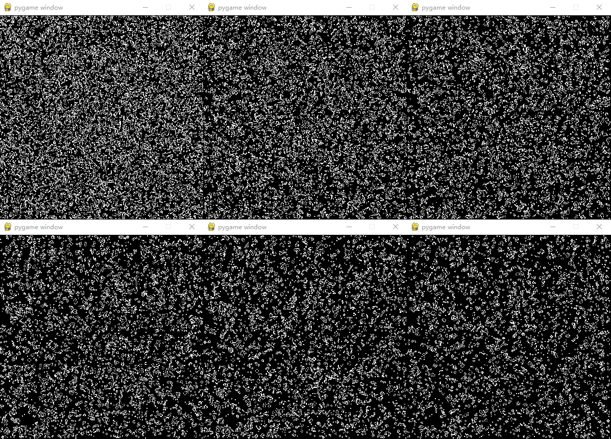
The above code sets a world of 400*400=16000 pixels, meaning 16000 lives. In each simulation round, the system queries the state of 16000 lives and their 8 surrounding neighbors, setting the simulation to stop after 100 rounds and outputting the time taken. It can be seen that the smoothness of the display is very poor, feeling like watching a PowerPoint presentation.
As we know, Python is an interpreted language, and during execution, its interpreter automatically determines the variable types, which increases the number of determinations in nested for loops, causing a rapid decline in performance. Therefore, Python is indeed not suitable for large-scale simulations. However, it is important to understand that many data analysis libraries in Python are written in C, such as NumPy, so its performance in data analysis remains good. The execution efficiency of C is much faster than that of Python. As a language closer to machines than humans, its complexity is also much higher than that of Python. To combine Python’s “humanity” and C’s high efficiency (machine execution efficiency), Cython was born. Cython is a library for Python, with its underlying code written in C, and it has its own compiler. Its greatest advantage is that it allows seamless addition of Cython code in Python, and its compiler translates Python code into C code for high-efficiency execution. In fact, pure Python code can also significantly improve performance after being translated and processed by Cython. In Jupyter Notebook, simply adding “%%cython” at the top of the code can boost speed by 20%.
To further leverage the advantages of Cython, we explicitly define the types of all variables that can have clear types, as shown in the following code.
%%cython
import time
import pygame, sys
from pygame.locals import *
import random
import numpy

cdef int HEIGHT = 400
cdef int WIDTH =400
WHITE = (255, 255, 255)
BLACK = (0,0,0)
cdef int FPS = 100
#cdef numpy.ndarray pxarray_orig
pygame.init()
fpsClock = pygame.time.Clock()
screen = pygame.display.set_mode((HEIGHT, WIDTH))
screen.fill(BLACK)
pxarray_orig = numpy.array(pygame.PixelArray(screen.copy()))
pxarray_orig = pygame.PixelArray(screen.copy())
cdef int i
cdef int j
cdef my_state
cdef init_color_value
cdef list neib_position
cdef int neighbor_state

for i in range(1,WIDTH-1):
    for j in range(1,HEIGHT-1):
        if random.randrange(2) < 1:
            screen.fill(0,((i,j),(1,1)))
        else:
            screen.fill(16777215,((i,j),(1,1)))

screen_new = screen.copy()
pygame.display.update()
cdef x = 0
startTime = time.time()
while x<100: # main game loop
    pxarray_orig = pygame.PixelArray(screen.copy())
    pxarray_new = pygame.PixelArray(screen.copy())
    init_color_value =  16777215

    for i in range(1,WIDTH-1):
        for j in range(1,HEIGHT-1):
            my_state = pxarray_orig[i,j]
            neib_position = [[i,j+1],[i,j-1],[i+1,j],[i-1,j],[i+1,j+1],[i-1,j-1],[i+1,j-1],[i-1,j+1]]
            neighbor_state = 0
            for position in neib_position:
                neighbor_state += pxarray_orig[position[0],position[1]]
            if my_state ==  16777215 and (neighbor_state == init_color_value*2 or neighbor_state==init_color_value*3):
                pxarray_new[i,j] = 16777215
            elif  my_state ==  16777215 and neighbor_state > init_color_value *3:
                pxarray_new[i,j] = 0
            elif my_state ==  16777215 and neighbor_state < init_color_value*2:
                pxarray_new[i,j] = 0
            elif my_state == 0 and neighbor_state==init_color_value*3:
                pxarray_new[i,j] = 16777215

    screen_new = pygame.PixelArray.make_surface(pxarray_new).copy()
screen.blit(screen_new,screen.get_rect().topleft)
pygame.display.flip()
    for event in pygame.event.get():
        if event.type == QUIT:
            pygame.quit()
            sys.exit()
    fpsClock.tick(FPS)
x += 1
executionTime = (time.time() - startTime)
print('Execution time in seconds: ' + str(executionTime))
pygame.quit()
The output is:
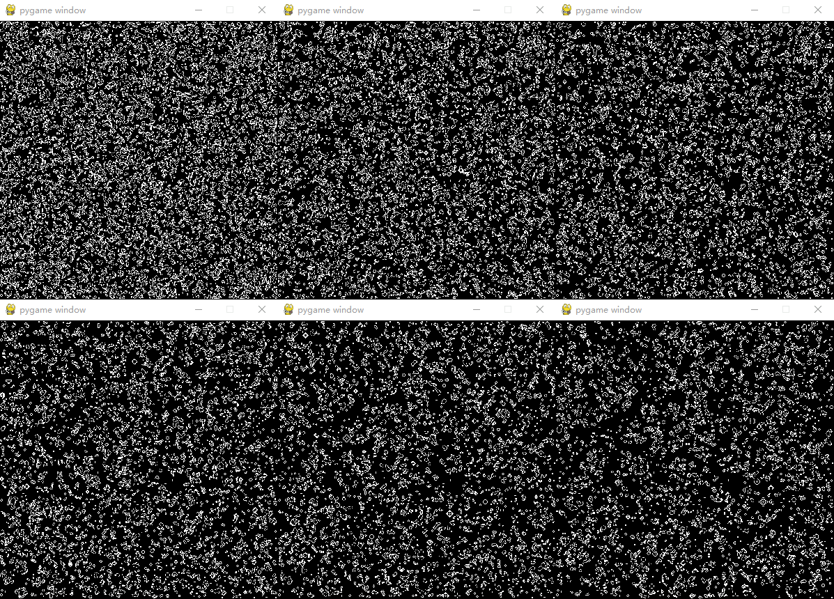
It has been tested that the speed of the above code has increased by about 100%! Of course, this significantly improves the smoothness of the display, but there is still a noticeable lag. However, the above code only adds variable type definitions compared to pure Python code. According to Cython’s claims, it provides not just half the performance of C, but nearly identical performance. Since we cannot directly define the internal data types of Pygame, we currently cannot fully leverage all the advantages of Cython.
To achieve smoother visuals, we can try implementing the Game of Life in C++. C++ is the development language for many large game engines and has significant advantages in fluid simulation and soft body simulation. Many large-scale agent-based modeling requires the use of supercomputers, and the implementation language for its models must be C++, not Python or JAVA.
This article presents two implementations in C++, one using vectors with pointers to control pixels, and the other using references to structures. Tests show that both methods have similar smoothness in display.
The implementation using vectors with pointers is as follows:
#include <SFML/Graphics.hpp>

const int WIDTH = 600, HEIGHT=600;
//template <typename Point>
const sf::Color WHITE = sf::Color(255, 255, 255, 255);
const sf::Color BLACK = sf::Color(0, 0, 0, 255);


class ParticleSystem : public sf::Drawable, public sf::Transformable
{
public:

    ParticleSystem(unsigned int count) :
        m_vertices(sf::Points, count)
    {
    }
    void generate_particle_matrix(int count)
    {
        std::vector<sf::Color> m_color_row;
        std::vector<sf::Vertex *> m_particle_row;
        for (int j = 0; j < HEIGHT; ++j) {
            m_particle_row.clear();
            m_color_row.clear();
            for (int k = 0; k < WIDTH; ++k) {
                sf::Vertex *p = &m_vertices[j * WIDTH + k];
                sf::Vector2f position = { float(j),float(k) };
                (*p).position = position;
                if (std::rand() % 100 < 50) {
                    (*p).color = WHITE;
                }
                else {
                    (*p).color = BLACK;
                }

                m_particle_row.push_back(p);
                m_color_row.push_back((*p).color);
            }
            m_particle_matrix.push_back(m_particle_row);
            m_particle_colors.push_back(m_color_row);

        }

    }


    void update()
    {
        for (int j = 1; j < HEIGHT - 1; ++j) {
            for (int k = 1; k < WIDTH - 1; ++k) {
                m_particle_colors[j][k] = (*m_particle_matrix[j][k]).color;
            }
        }

        for (int j = 1; j < HEIGHT-1; ++j) {
            for (int k = 1; k < WIDTH-1; ++k) {
                int neighbor_position[8][2] = { {j,k + 1}, {j,k - 1}, {j + 1,k}, {j + 1,k + 1}, {j + 1,k - 1}, {j - 1,k}, {j - 1,k + 1}, {j - 1,k - 1} };
                sf::Color&& my_color = (*m_particle_matrix[j][k]).color;
                int color_count = 0;
                for (int l = 0; l < 8;++l) {
                    if (m_particle_colors[neighbor_position[l][0]][neighbor_position[l][1]] == WHITE){
                        color_count++;
                    }
                }

                if (my_color == WHITE && (color_count == 2 || color_count==3)) {
                    my_color = WHITE;

                }
                else if (my_color == WHITE && color_count>3) {
                    my_color = BLACK;

                }
                else if (my_color == WHITE && color_count < 2) {
                    my_color = BLACK;
                }
                else if (my_color == BLACK && color_count == 3) {
                    my_color = WHITE;
                }
            }
        }
    }

private:

    virtual void draw(sf::RenderTarget&& target, sf::RenderStates states) const
    {
        states.transform *= getTransform();

        states.texture = NULL;

        target.draw(m_vertices, states);
    }

private:

    struct Particle
    {
        sf::Vector2f velocity;
        sf::Time lifetime;
    };

     sf::VertexArray m_vertices;
     std::vector<std::vector<sf::Vertex*>> m_particle_matrix;
     std::vector<std::vector<sf::Color>> m_particle_colors;

};

int main()
{

    sf::RenderWindow window(sf::VideoMode(WIDTH, HEIGHT), "Life Game");

    ParticleSystem particles(WIDTH*HEIGHT);
    particles.generate_particle_matrix(WIDTH*HEIGHT);

    sf::Clock clock;


    while (window.isOpen())
    {

        sf::Event event;
        while (window.pollEvent(event))
        {
            if (event.type == sf::Event::Closed)
                window.close();
        }

        particles.update();
        window.clear();
        window.draw(particles);
        window.display();
    }

    return 0;
}
The implementation using structures with references is as follows:
#include <SFML/Graphics.hpp>

const int WIDTH = 500, HEIGHT = 500;
const sf::Color WHITE = sf::Color(255, 255, 255, 255);
const sf::Color BLACK = sf::Color(0, 0, 0, 255);


class ParticleSystem : public sf::Drawable, public sf::Transformable
{
public:

    ParticleSystem(unsigned int count) :
        m_particles(count),
        m_vertices(sf::Points, count)
    {
    }
    void generate_particle_matrix(int count)
    {
        for (int j = 0; j < HEIGHT; ++j) {
            for (int k = 0; k < WIDTH; ++k) {
                sf::Vector2f position = { float(j),float(k) };
                Particle&& p = m_particles[j * WIDTH + k];
                sf::Vertex&& v = m_vertices[j * WIDTH + k];
                p.position = position;
                v.position = p.position;
                if (std::rand() % 100 < 50) {
                    p.my_color = WHITE;
                }
                else {
                    p.my_color = BLACK;
                }
                v.color = p.my_color;
            }
        }
    }

    void update()
    {
        for (int j = 0; j < HEIGHT; ++j) {
            for (int k = 0; k < WIDTH; ++k) {
                if (j - 1 > 0 && j + 1 < HEIGHT && k - 1 > 0 && k + 1 < WIDTH) {
                    Particle&& p = m_particles[j * (WIDTH)+k];
                    sf::Vertex&& v = m_vertices[j * (WIDTH)+k];
                    int neighbor_position[8] = { j*WIDTH+k + 1, j*WIDTH+k - 1, (j + 1)*WIDTH+k,
                        (j + 1)*WIDTH+k + 1, (j + 1)*WIDTH+k - 1, (j - 1)*WIDTH+k, (j - 1)*WIDTH+k + 1, (j - 1)*WIDTH+k - 1};
                    int color_count = 0;
                    for (int l = 0; l < 8; ++l) {
                        if (m_vertices[neighbor_position[l]].color == WHITE) {
                            color_count++;
                        }
                    }

                    if (v.color == WHITE && (color_count == 2 || color_count == 3)) {
                         p.my_color = WHITE;
                        }
                        else if (v.color == WHITE && color_count > 3) {
                            p.my_color = BLACK;
                        }
                        else if (v.color == WHITE && color_count < 2) {
                            p.my_color = BLACK;
                        }
                        else if (v.color == BLACK && color_count == 3) {
                            p.my_color = WHITE;
                        }
                }
            }
        }

        for (int i = 0; i < WIDTH * HEIGHT; ++i) {
            m_vertices[i].color = m_particles[i].my_color;
        }
    }


private:

    virtual void draw(sf::RenderTarget&& target, sf::RenderStates states) const
    {
        states.transform *= getTransform();

        states.texture = NULL;

        target.draw(m_vertices, states);
    }

private:

    struct Particle
    {
        sf::Vector2f position;
        sf::Color my_color;
    };

    std::vector<Particle> m_particles;
    sf::VertexArray m_vertices;
    std::vector<std::vector<sf::Vertex*>> m_particle_matrix;
    std::vector<std::vector<sf::Color>> m_particle_colors;

};

int main()
{

    sf::RenderWindow window(sf::VideoMode(WIDTH, HEIGHT), "Life Game");

    ParticleSystem particles(WIDTH * HEIGHT);
    particles.generate_particle_matrix(WIDTH * HEIGHT);

    sf::Clock clock;

    while (window.isOpen())
    {
        sf::Event event;
        while (window.pollEvent(event))
        {
            if (event.type == sf::Event::Closed)
                window.close();
        }

        particles.update();
        window.clear();
        window.draw(particles);
        window.display();
    }

    return 0;
}
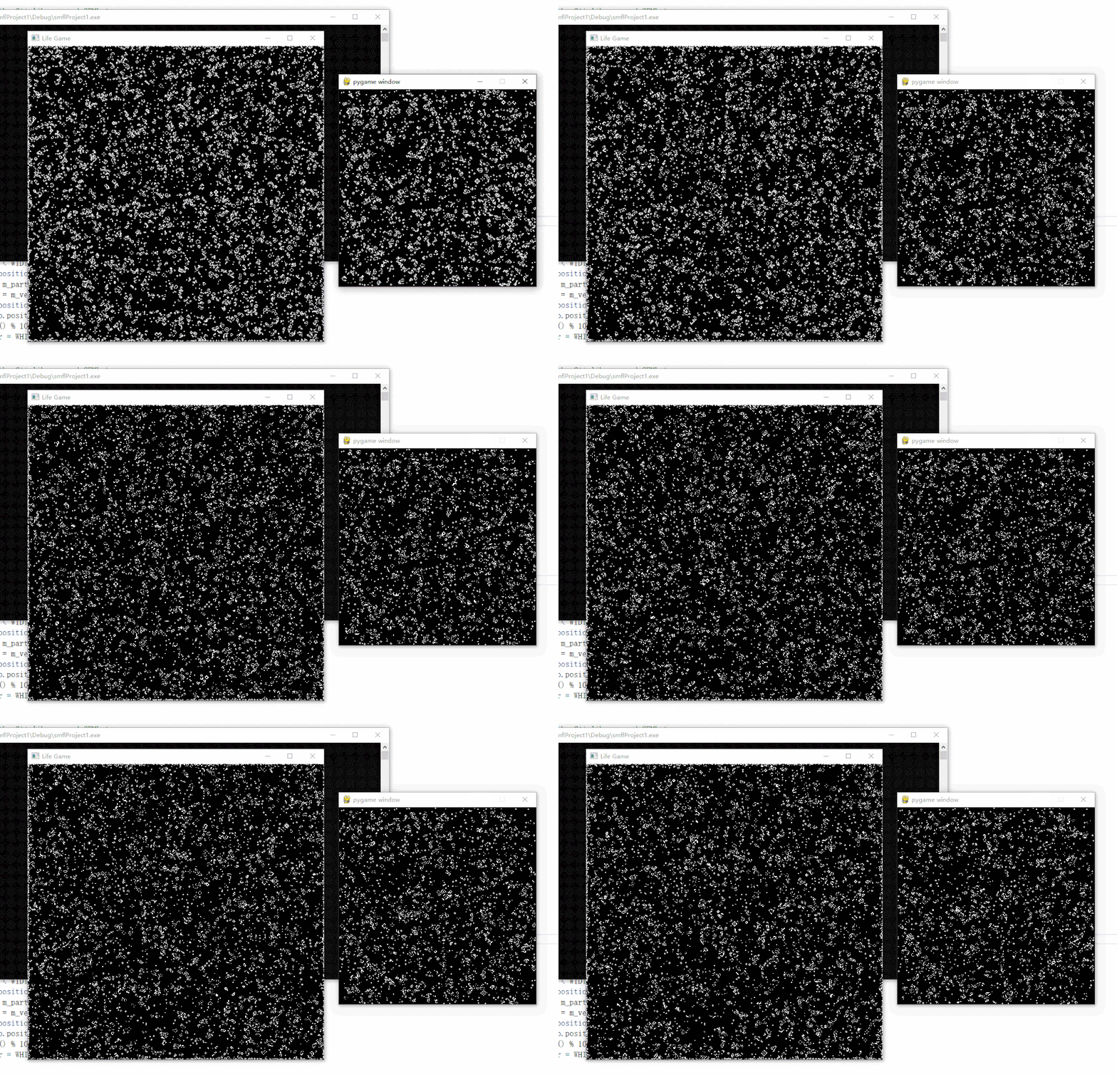
To compare the output effects of C++ and Python, we will place the outputs of both side by side, where the Python code has already been compiled with Cython. Below is a comparison of the effects of different pixels between the two. Although the animated GIF screenshots also have their FPS limitations, it can still be seen that even after Cython compilation, the smoothness of Python is still far below that of C++.
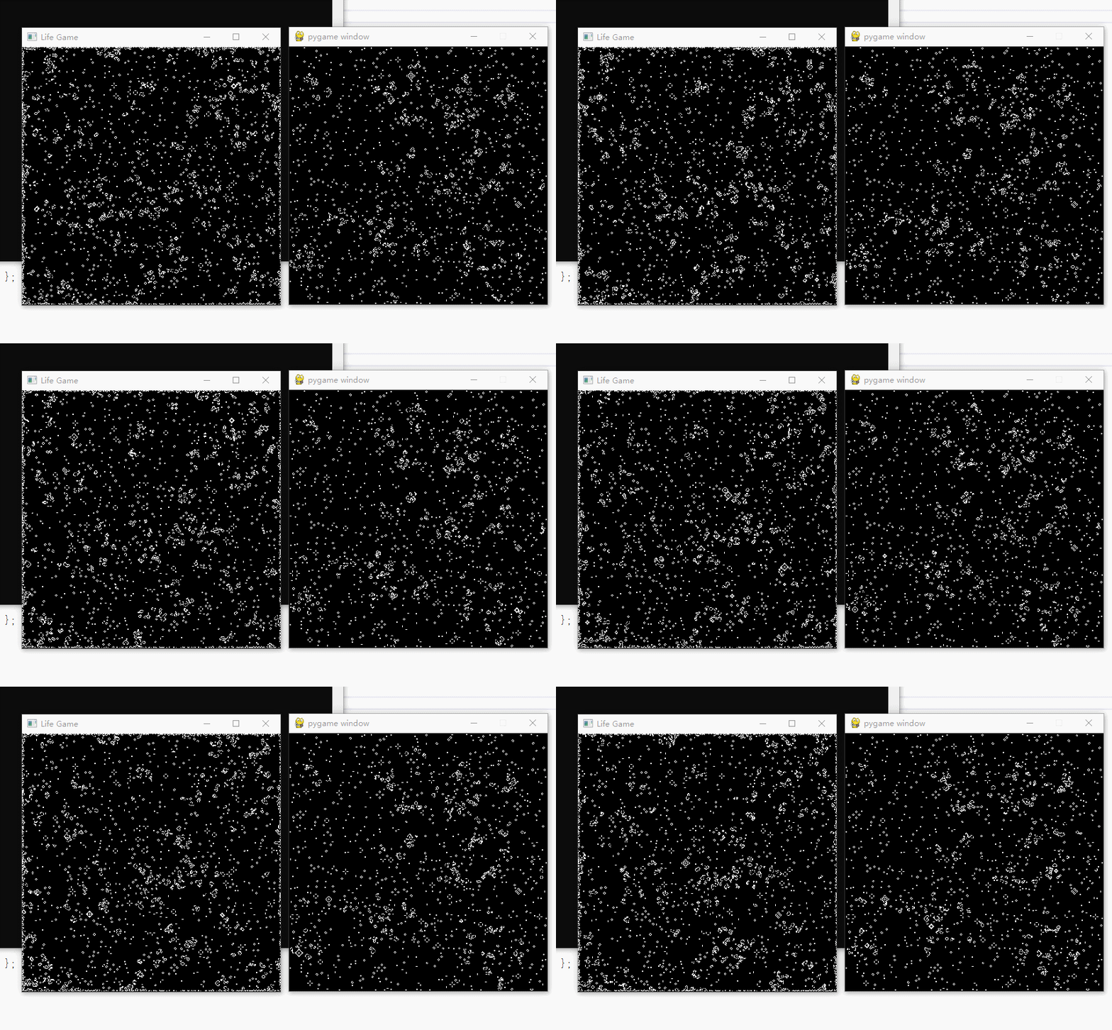
C++400*400 VS Python400*400
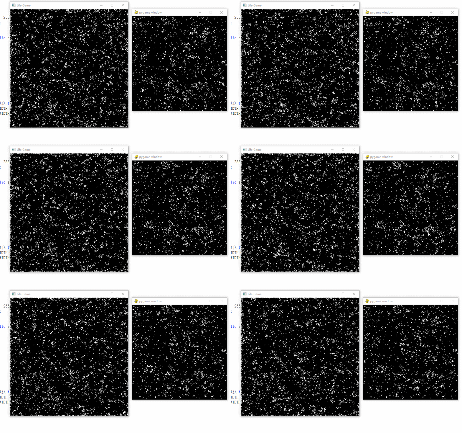
C++500*500 VS Python 400*400
C++600*600 VS Python 400*400
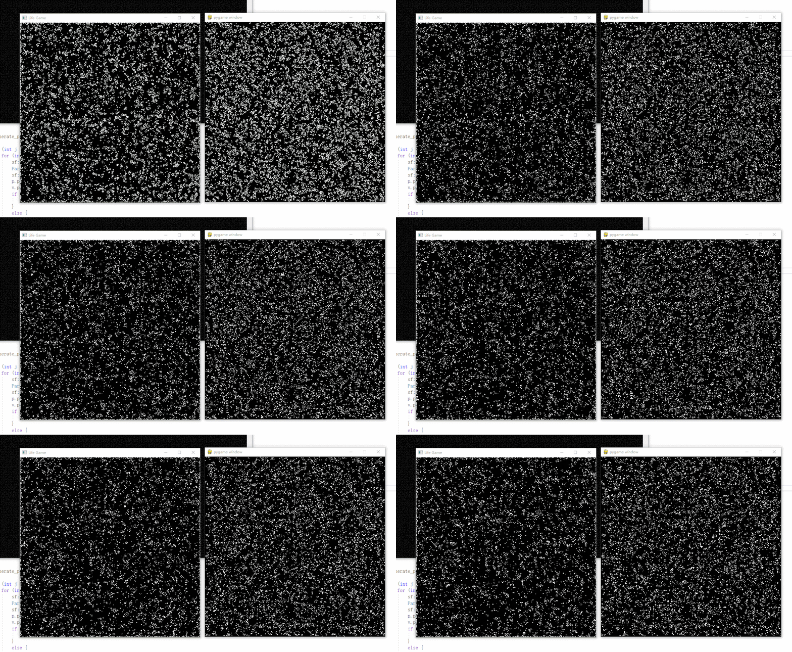
It can be seen that even when processing 600*600 pixels, the smoothness of C++ still exceeds that of Python processing 400*400. Python shows a clear struggle at 600*600 pixels.
Conclusion:
C++ is indeed a language that supports supercomputing, far surpassing Python in handling large-scale simulation entities. However, Python’s dominant position in data analysis and artificial intelligence still gives it a significant ecological advantage. Therefore, if the model needs to handle large-scale issues and has high demands for dynamic visualization, C++ can be used for implementation; meanwhile, Python can serve as the main tool for data analysis. Additionally, Python can be used for the development and exploration of model prototypes, as its development efficiency and difficulty are much lower than that of C++. Thus, both languages have their unique advantages in modeling, and one should leverage each other’s strengths during the modeling process.
Note: The entire text is reproduced from Scientific Modeling DrZ‘s Toutiao column