
Prelude
Mathematical Foundations
1. Functions
A function is a type of mapping relationship (correspondence/rule).
Since it is a mapping relationship, there must be at least two numbers, one of which participates in the mapping, while the other number establishes a relationship with the mapping result.
Typically, we use x and y to represent the two numbers, with x participating in the mapping and y establishing a relationship with the mapping result.
Mapping is essentially a formula (rule) that uses x to participate in the calculation.
The relationship is simply a comparison of sizes (logic), where there are four possible comparisons of two values: greater than, less than, equal to, and not equal to.
[Example 1]
Using “2x+1” as the mapping rule, and using “equals” to indicate the relationship between y and the mapping result,
the function can be expressed as: y = 2x + 1.
[Example 2]
Using “x(x+1)+2” as the mapping rule, and using “equals” to indicate the relationship between y and the mapping result,
the function can be expressed as: y = x(x + 1) + 2.
For the above two functions, for each given value of x, there will be a corresponding y, and y changes as x changes, so x is called the independent variable, y is called the dependent variable, the range of x is called the domain, and the range of y is called the range.
When y is equal to the mapping result, y is also called the function value.
The domain, range, and the mapping rule together constitute the three essential elements of a function.
In addition to using y to represent the function of x, we can also use f(x) to replace y to express the function of x.
Thus, the above two functions can also be expressed as follows:
f(x) = 2x + 1
f(x) = x(x + 1) + 2
2. Function Graphs
Having learned about functions, it is essential to learn about function graphs because the combination of numbers and shapes is the essence of science and the best description of nature, allowing people to appreciate the beauty and charm of mathematics.
The famous mathematician Hua Luogeng once said: “When numbers lack shapes, they are less intuitive; when shapes lack numbers, they are difficult to analyze in detail.” This emphasizes the importance of the combination of numbers and shapes in mathematical learning and research.
The function graph is the image depicted in the Cartesian coordinate system for each pair of independent and dependent variables, that is, the image composed of each pair of (x, y) coordinate points.
Here is a great website for observing different function graphs:
Function Graph Viewer Tool
https://www.geogebra.org/graphing
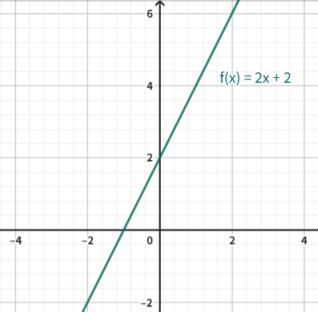
The graph of the function: y = 2x + 2 is shown below:
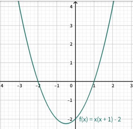
The graph of the function: y = x(x + 1) + 2 is shown below:
【Thought】Inequalities
1. If the above two functions change the equality relationship to greater than, less than, or not equal, what changes occur in the graph regions represented?
2. If we directly establish an equality relationship between the two functions, that is:2x + 2 = x(x + 1) + 2, what region does the graph represent?
3. What regions do 2x + 2 > x(x + 1) + 2 and 2x + 2 < x(x + 1) + 2 represent respectively?
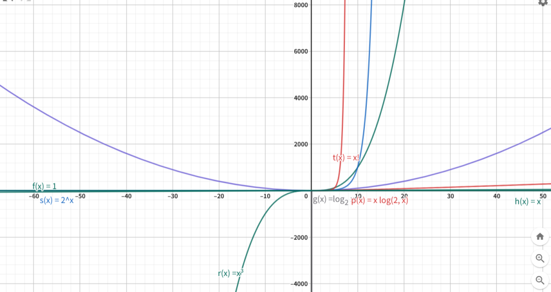
Common algorithm complexity function graphs are shown below: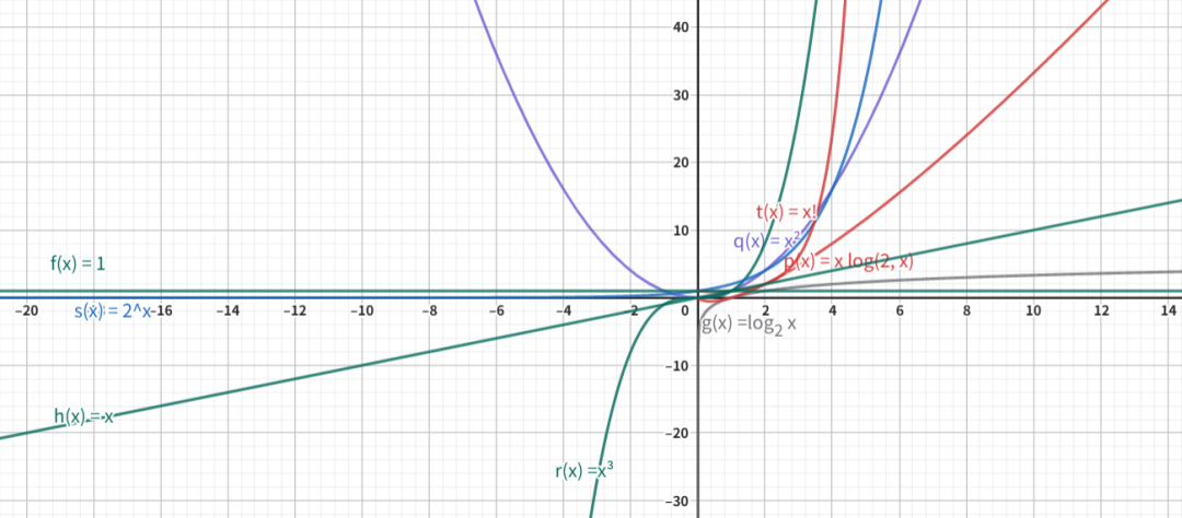
3. Logarithms
1. The concept of logarithms: Generally, if a^x = N (a>0 and a!=1), then the number x is called the logarithm of N to the base a, denoted as: x = loga N. Here, a is called the base, and N is called the argument. It can be understood as: logarithms are operations to solve for the exponent when the base and the power are known.
[Example 1]
Since 2^3 = 8, the logarithm of 8 to the base 2 is 3, denoted as: log2 8 = 3.
[Example 2]
Since 2^x = 32, the logarithm of 32 to the base 2 is x, denoted as: x = log2 32.
2. Basic properties of logarithms:
(1) Negative numbers and 0 have no logarithm. Because the base a is greater than 0, a^x is always greater than 0.(2) The logarithm of 1 is 0. Because a^0 = 1, any positive number raised to the power of 0 is 1.(3) The logarithm of the base is 1. Because a^1 = a, any positive number raised to the power of 1 is itself.(4) Logarithmic identity 1: a ^ loga N = N (a>0 and a!=1, N>0).(5) Logarithmic identity 2: loga a^b = b (a>0 and a!=1).
3. Properties of logarithmic operations:
(1) loga (M·N) = loga M + loga N.(2) loga (M/N) = loga M – loga N.(3) loga M^n = n·loga M.
1
Overview
Generally speaking, there are multiple algorithms available to solve the same problem (such as bubble sort, insertion sort, bucket sort, etc.), how do we measure the pros and cons of each algorithm?
Even when using the same algorithm to solve the same problem, due to hardware limitations, differences in programming languages, and variations in test data volume, the evaluation results can vary significantly.
To objectively and scientifically measure the quality of algorithms, we can use algorithm complexity for analysis and consideration.
Algorithm complexity is an important indicator of algorithm efficiency; it does not concern specific test data but focuses on the growth trend of the resources required (time and space) as the data scale (n) increases.
Since the focus is on trends, it will not be very precise, so algorithm complexity is a rough estimate of algorithm execution efficiency.
[Characteristics of Algorithm Complexity]
- Objectivity: Not influenced by external factors, objective and scientific;
- Standardization: A theoretical measurement standard that can compare the pros and cons of different algorithms.
[Classification/Dimensions of Algorithm Complexity]1. Time Complexity: The relationship between the time required for algorithm execution and the data scale, describing the speed of problem-solving;2. Space Complexity: The relationship between the storage space required for algorithm execution and the data scale, describing the degree of storage space occupied during problem-solving.A good algorithm should solve problems as quickly as possible while using as little storage space as possible.
2
Representation Methods
Big O Notation:
Big O notation uses the uppercase letter “O” to represent the upper bound of algorithm complexity (the growth trend in the worst case). We care about the order of magnitude, not the exact number of steps.
If we denote f(n) as a function of input size n, then O(f(n)) represents the algorithm’s complexity.
For the following functions of size n:
f(n) = 3
f(n) = n + 1
f(n) = n^2 + n + 10
f(n) = 5n^123 - 100n + 100
According to the following rules:
If there are only constant terms, use O(1) to represent algorithm complexity.
If there are multiple terms added together, only take the term with the largest order of magnitude, and remove coefficients and other terms.
The algorithm complexities are represented as follows:
O(1)
O(n)
O(n^2)
O(n^123)
Common levels of algorithm complexity (from best to worst):
| Complexity | Name | Examples |
| O(1) | Constant Order | Accessing array elements, hash table lookup |
| O(log n) | Logarithmic Order | Binary search, balanced binary search tree operations |
| O(n) | Linear Order | Traversing arrays, searching for elements in linked lists |
| O(n log n) | Linear Logarithmic Order | Efficient sorting algorithms (quick, merge, bucket sort) |
| O(n^2) | Quadratic Order | Simple sorting algorithms (bubble, selection, insertion) |
| O(n^3) | Cubic Order | Multiplying two n-order matrices |
| O(2^n) | Exponential Order | Tower of Hanoi problem, exhaustive search (brute force) |
| O(n!) | Factorial Order | Finding all permutations of n elements |
From the above table, I believe everyone can understand: Why learn bubble sort if you also learn quick sort? Why learn arrays if you also learn data structures?[Exercise 1] Write down the algorithm complexity of the following polynomials (1) 5·n^2 + 10·n + 100 (2) n^3 / 1000 + 2^n (3) 200 + 1 / n (4) log n^5 + 3.14 (5) 3·log 3^n [Exercise 1] Reference Answers (1) O(n^2) (2) O(2^n) (3) O(1) (4) O(log n) (5) O(n)
3
Calculating Algorithm Complexity
Method 1: Forward Substitution Method
Example 1:
Given the following recurrence relation, find the algorithm complexity.
f(n) = 2 f(n-1) + 1, f(1) = 1.
Method:
Substituting from f(1) to f(n) step by step, calculating forward, and finding patterns from the results.
Steps:
1. f(1) = 1
2. f(2) = 2 f(1) + 1 = 2 * 1 + 1 = 3
3. f(3) = 2 f(2) + 1 = 2 * 3 + 1 = 7
4. f(4) = 2 f(3) + 1 = 2 * 7 + 1 = 15
5. f(5) = 2 f(4) + 1 = 2 * 15 + 1 = 31
……
Summarizing the pattern:
1. f(1) = 2^1 – 1
2. f(2) = 2^2 – 1
3. f(3) = 2^3 – 1
4. f(4) = 2^4 – 1
5. f(5) = 2^5 – 1
……
Conclusion:
f(n) = 2^n – 1
Therefore, the algorithm complexity of the above recurrence relation is: O(2^n).
Method 2: Backward Substitution Method
Example 2:
Given the following recurrence relation, find the algorithm complexity.
f(n) = f(n-1) + n, f(0) = 0.
Method:
Substituting from f(n) to f(0) step by step, calculating backward, and finding patterns from the results.
Steps:
f(n) = f(n-1) + n = f(n-2) + (n-1) + n = f(n-3) + (n-2) + (n-1) + n …… = f(0) + 1 + 2 + 3 + …… + (n-1) + n = 0 + 1 + 2 + 3 + …… + (n-1) + n = n(n+1)/2Conclusion:
f(n) = n(n+1) / 2 = n^2 / 2 + n / 2
Therefore, the algorithm complexity of the above recurrence relation is: O(n^2).
4
Analysis of Code Complexity
Method 1: Addition Rule
The total complexity of the code equals the complexity of the segment with the largest order of magnitude.
Example 1: Analyze the time complexity of the following code
int test_11(int n) {
    int sum_1 = 0;
    for (int i = 1; i <= 100; ++i) {  // Calculation times: 100
        sum_1 = sum_1 + i;
    }   // O(1)
    int sum_2 = 0;
    for (int i = 0; i <= n; ++i) {  // Calculation times: n + 1
        sum_2 += i;  // O(n)
    }
    int sum_3 = 0;
    for (int i = 1; i <= n; i++) {  // Calculation times: n
        for (int j = 1; j <= n; j++) {  // Calculation times: n
            sum_3 += i * j;  // Calculation times: n^2
        }
    }   // O(n^2)
    return sum_1 + sum_2 + sum_3;  // Total calculation times: 100 + n + 1 + n^2
}   // Overall time complexity: O(n^2)
The above function mainly consists of three for loops, the first for loop has a calculation count of 100, the second for loop executes n+1 times, and the third for loop is a nested loop, where each layer of the loop executes n times, resulting in a total of n^2 executions.
According to the addition principle, we choose the segment with the largest order of magnitude (i.e., the third nested for loop) as the time complexity of the entire function.
Example 2: Analyze the time complexity of the following code
int test_12(int m, int n) {
    int sum_1 = 0;
    for(int i = 1; i <= m; i++) {
        sum_1 += i;
    }
    int sum_2 = 0;
    for(int j = 1; j <= n; j++) {
        sum_2 += j;
    }
    return sum_1 + sum_2;
}
The above function mainly consists of two for loops, each of which is a single-layer loop.
The first for loop has a loop count of m, with a time complexity of: O(m),
The second for loop has a loop count of n, with a time complexity of: O(n).
The overall function’s calculation count is: m + n, with a time complexity of: O(m + n).
Summary:
When there are parallel loops, and the powers of each loop’s count are the same but cannot be compared, the complexities of each loop are added together to determine the overall function’s time complexity.
Method 2: Multiplication Rule
The complexity of nested code equals the product of the complexities of each layer of nesting.
Example 1: Analyze the complexity of the following code
int f_21(int n) {
    int sum = 0;
    for (int i = 1; i <= n; ++i) {
        sum += i;
    }
    return sum;
}
int test_21(int n) {
    int ret = 0;
    for (int i = 1; i <= n; ++i) {
        ret += f_21(i);
    }
    return ret;
}
The function f_21 mainly consists of 1 single-layer for loop, with a calculation count of: n, so the time complexity of function f_21 is: O(n);
The function test_21 also consists of 1 single-layer for loop, with a calculation count of: n, so is the time complexity of function test_21 also O(n)?
Clearly, test_21 is not that simple. Because in each iteration of test_21, f_21 is called once, and each call to f_21 requires i operations.
Although function test_21 also loops n times, the number of operations executed in each round of the loop varies: the first round executes 1 operation, the second round executes 2 operations, the third round executes 3 operations… the nth round executes n operations.
Calculation count = 1 + 2 + 3 + …… + n = n(n + 1) / 2 = n^2 / 2 + n / 2Therefore, the time complexity of test_21 is: O(n^2).
Summary:
test_21’s for loop is the outer loop, with a time complexity of: O(n),
f_21’s for loop is the inner loop, with a time complexity of: O(n),
The final time complexity of test_21 equals the product of the complexities of the inner and outer nested loops,
i.e., O(n) * O(n) = O(n * n) = O(n^2).
5
Time Complexity Examples
Generally, the time complexity is measured by the number of steps executed by the algorithm; the more steps executed, the more time consumed, and vice versa, the less time used.
Therefore, the time complexity can be determined based on the number of steps executed by the algorithm.
Example 1: Constant Time Complexity O(1)
// Accessing array elements
int getElement(int arr[], int index) {
    return arr[index];     // O(1)
}
// Simple mathematical operation
int sum(int a, int b) {
    return a + b;         // O(1)
}
Example 2: Linear Time Complexity O(n)
// Traversing an array to sum
int arraySum(int arr[], int n) {
    int sum = 0;
    for (int i = 0; i < n; i++) {  // O(n)
        sum += arr[i];             // O(1)
    }
    return sum;                    // O(1)
} // Total complexity: O(n)
Example 3: Quadratic Time Complexity O(n^2)
// Bubble sort
void bubbleSort(int arr[], int n) {
    for (int i = 0; i < n-1; i++) {         // O(n)
        for (int j = 0; j < n-i-1; j++) {   // O(n)
            if (arr[j] > arr[j+1]) {        // O(1)
                swap(arr[j], arr[j+1]);     // O(1)
            }
        }
    }}// Total complexity: O(n²)
Example 4: Logarithmic Time Complexity O(log n)
// Binary search
int binarySearch(int arr[], int left, int right, int target) {
    while (left <= right) {
        int mid = left + (right - left) / 2;    // O(1)
        if (arr[mid] == target)                 // O(1)
            return mid;
        else if (arr[mid] < target)             // O(1)
            left = mid + 1;
        else
            right = mid - 1;                    // O(1)
    }
    return -1;
}// Each iteration halves the search range: O(log n)
Example 5: Linear Logarithmic Time Complexity O(n log n)
// Merge operation in merge sort
void merge(int arr[], int left, int mid, int right) {
    // Merging two sorted arrays: O(n)}
void mergeSort(int arr[], int left, int right) {
    if (left < right) {
        int mid = left + (right - left) / 2;  // O(1)
        mergeSort(arr, left, mid);           // T(n/2)
        mergeSort(arr, mid+1, right);        // T(n/2)
        merge(arr, left, mid, right);        // O(n)
    }}// Recursive depth: O(log n), each merge: O(n)// Total complexity: O(n log n)
6
Space Complexity Examples
Example 1: Constant Space Complexity O(1)
// In-place swap
void swap(int &a, int &b) {
    int temp = a;  // Only uses a fixed amount of extra space
    a = b;
    b = temp;
}
Example 2: Linear Space Complexity O(n)
// Fibonacci sequence (recursive, inefficient version)
int fibonacci(int n) {
    if (n <= 1) return n;
    return fibonacci(n-1) + fibonacci(n-2);    // Call stack depth: O(n)
}
// Creating a one-dimensional array
int n;
cin >> n;
vector<int> arr(n);  // O(n) space
for (int i = 0; i < n; i++) {
    cin >> arr[i];
}
< This lesson ends here >
Previous Recommendations
C++ Programming for Kids (18) Bit Manipulation
C++ Programming for Kids (17) High-Precision Algorithms (Multiplication and Division)
C++ Programming for Kids (16) High-Precision Algorithms (Addition and Subtraction)
C++ Programming for Kids (15) Divide and Conquer Algorithms
C++ Programming for Kids (14) Recursive Algorithms
C++ Programming for Kids (13) Iterative Algorithms
C++ Programming for Kids (12) Sorting Algorithms (4) Counting Sort
200 – Eliminate the Enemy (J)
Python Programming for Kids (20) Divide and Conquer Algorithms
Python Programming for Kids (19) Recursion and Iteration
Scratch Version of “Gold Miner” (Paid)
J30-01 Knapsack Problem (Dynamic Programming)
Visual Training Mini Game – Fox Doodle (Paid)
J29 – Tower of Hanoi (Divide and Conquer)
Visual Training Mini Game – Find Text (Paid)


Scan the QR code to get
More Exciting Content
Little Xiao Kids Programming