Building a Fusion Model of Transformer and Wavelet Transform for Univariate Time Series Prediction (Case Study + Source Code)

This is my423rd original article.

Introduction

“Data Forum” focuses on Python as the core, vertical to the data science field, specializing in (click 👉) Python programming development | data collection | data analysis | data visualization | feature engineering | machine learning | time series data | deep learning | artificial intelligence and other technology stacks for communication and learning, covering data mining, computer vision, natural language processing and other application fields. (There is a surprise at the end benefits.)

1. Introduction

Fusion Method of Transformer and Wavelet Transform

1. Perform wavelet decomposition on the original time series to obtain different frequency components;
2. Input multiple components as multi-channel inputs into the Transformer;
3. The Transformer learns the temporal relationships between different frequency bands.

By using wavelets to extract “frequency features” and then using the Transformer to extract “sequence dependencies”, or introducing wavelet concepts into the attention mechanism, the model becomes more suitable for complex time series prediction tasks.

2. Implementation Process

2.1 Data Reading

Core code:

data = pd.read_csv('data.csv')# Convert date column to datetime type
data['Month'] = pd.to_datetime(data['Month'])# Set date column as index
data.set_index('Month', inplace=True)
data = np.array(data['Passengers'])
T = len(data)
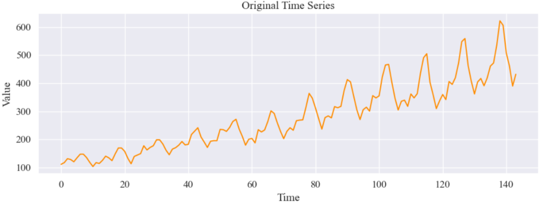
x = np.arange(len(data))# Visualization: Original time series
plt.figure(figsize=(10, 4))
plt.plot(x, data, color='darkorange')
plt.title('Original Time Series')
plt.xlabel('Time')
plt.ylabel('Value')
plt.grid(True)
plt.tight_layout()
plt.show()

Result:

2.2 Wavelet Decomposition and Normalization Processing

Core code:

wavelet = 'db4'
coeffs = pywt.wavedec(data, wavelet, level=2)
a2, d2, d1 = coeffs# Reconstruct original signal
low_freq  = pywt.waverec([a2, np.zeros_like(d2), np.zeros_like(d1)], wavelet)
mid_freq  = pywt.waverec([np.zeros_like(a2), d2, np.zeros_like(d1)], wavelet)
high_freq = pywt.waverec([np.zeros_like(a2), np.zeros_like(d2), d1], wavelet)
print(low_freq.shape, mid_freq.shape, high_freq.shape)# Uniform length
min_len = min(len(low_freq), T)
components = np.stack([low_freq[:min_len], mid_freq[:min_len], high_freq[:min_len]], axis=1)# Normalization
scaler = MinMaxScaler()
components_scaled = scaler.fit_transform(components)
target = data[1:1+min_len]  # Lag 2 steps for prediction to avoid data leakage

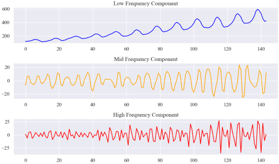
Using Daubechies-4 (db4) wavelet function for 2-level decomposition of the original data, extracting three types of information: low frequency (trend), mid frequency (period), and high frequency (noise). Each frequency component is reconstructed and aligned, forming a three-dimensional input feature, and then scaled to the range [0, 1] using MinMaxScaler to prevent model training instability.

The curve changes of the three frequency components: low frequency is stable, mid frequency has rhythmic changes, and high frequency oscillates violently, reflecting the multi-scale features contained in the data.

2.3 Constructing PyTorch Dataset

Core code:

window_size = 7
offset = 1   
dataset = TimeSeriesDataset(X_all, y_all, window_size)
train_size = int(len(dataset) * 0.8)
train_dataset, test_dataset = torch.utils.data.random_split(dataset, [train_size, len(dataset) - train_size])
train_loader = DataLoader(train_dataset, batch_size=32, shuffle=True)
test_loader = DataLoader(test_dataset, batch_size=32)

2.4 Transformer Model Design

Core code:

class WaveletTransformer(nn.Module):
    def __init__(self, input_dim, d_model=64, nhead=4, num_layers=2):
        super().__init__()
        self.linear_in = nn.Linear(input_dim, d_model)
        encoder_layer = nn.TransformerEncoderLayer(d_model=d_model, nhead=nhead, batch_first=True)
        self.transformer = nn.TransformerEncoder(encoder_layer, num_layers=num_layers)
        self.decoder = nn.Sequential(
            nn.Linear(d_model, 32),
            nn.ReLU(),
            nn.Linear(32, 1)
        )
    def forward(self, x):
        x = self.linear_in(x)
        x = self.transformer(x)
        x = x[:, -1, :]
        out = self.decoder(x).squeeze(-1)
        return out
model = WaveletTransformer(input_dim=3)

A Transformer model with two encoder layers has been constructed, with input being a three-dimensional time series (representing three frequency bands). The model structure includes: linear mapping, Transformer encoder (multi-head attention), and a regression decoder for predicting the true value of the next time point.

2.5 Model Training and Loss Analysis

Core code:

criterion = nn.MSELoss()
optimizer = optim.Adam(model.parameters(), lr=0.001)
epochs = 500
train_losses = []
test_losses = []
for epoch in range(epochs):
    model.train()
    total_loss = 0
    for X_batch, y_batch in train_loader:
        optimizer.zero_grad()
        output = model(X_batch)
        loss = criterion(output, y_batch)
        loss.backward()
        optimizer.step()
        total_loss += loss.item()
    train_losses.append(total_loss / len(train_loader))
    model.eval()
    with torch.no_grad():
        test_loss = sum(criterion(model(X), y).item() for X, y in test_loader) / len(test_loader)
        test_losses.append(test_loss)

Using mean squared error (MSE) as the loss function and Adam optimizer for 500 training epochs.

plt.figure(figsize=(8, 4))
plt.plot(train_losses, label='Train Loss', color='royalblue')
plt.plot(test_losses, label='Test Loss', color='tomato')
plt.title('Loss Curve')
plt.xlabel('Epoch')
plt.ylabel('MSE')
plt.legend()
plt.grid(True)
plt.tight_layout()
plt.show()

Result

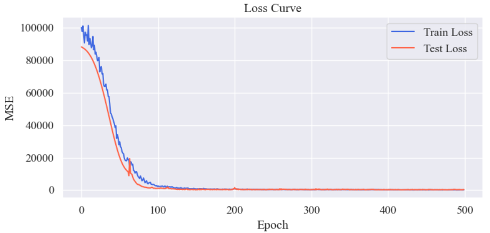
The visualization of the training process shows the loss curves for the training and test sets over epochs, both converging, indicating that the model is stable and not overfitting significantly.

2.6 Prediction Result Analysis and Visualization

Core code:

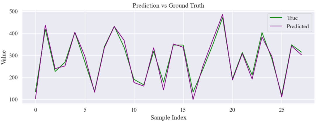
Using the test set for model inference, obtaining a comparison of true values and predicted values.

model.eval()
preds = []
y_true = []
with torch.no_grad():
    for X, y in test_loader:
        pred = model(X)
        preds.extend(pred.numpy())
        y_true.extend(y.numpy())

Prediction effect diagram clearly shows the model’s ability to predict future values, with the prediction curve closely fitting the true curve, indicating that the model has extracted effective features.

plt.figure(figsize=(10, 4))
plt.plot(y_true, label='True', color='green')
plt.plot(preds, label='Predicted', color='purple')
plt.title('Prediction vs Ground Truth')
plt.xlabel('Sample Index')
plt.ylabel('Value')
plt.legend()
plt.tight_layout()
plt.show()

Result:

The curve changes of the three frequency components: low frequency is stable, mid frequency has rhythmic changes, and high frequency oscillates violently, reflecting the multi-scale features contained in the data.

plt.figure(figsize=(10, 6))
plt.subplot(3, 1, 1)
plt.plot(components[:min_len, 0], color='blue')
plt.title('Low Frequency Component')
plt.subplot(3, 1, 2)
plt.plot(components[:min_len, 1], color='orange')
plt.title('Mid Frequency Component')
plt.subplot(3, 1, 3)
plt.plot(components[:min_len, 2], color='red')
plt.title('High Frequency Component')
plt.tight_layout()
plt.show()

Result:

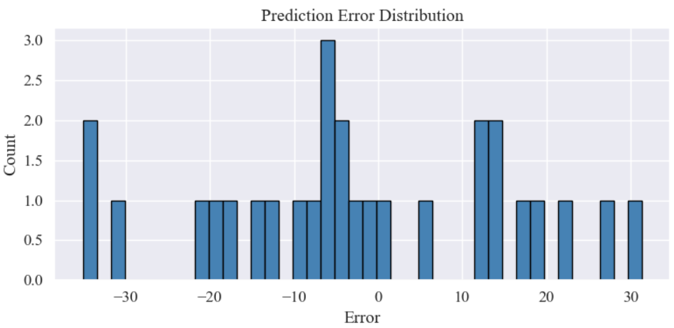
Prediction error distribution diagram:

errors = np.array(preds) - np.array(y_true)
plt.figure(figsize=(8, 4))
plt.hist(errors, bins=40, color='steelblue', edgecolor='black')
plt.title('Prediction Error Distribution')
plt.xlabel('Error')
plt.ylabel('Count')
plt.grid(True)
plt.tight_layout()
plt.show()

Result:

Conclusion

Author’s Biography:

During my graduate studies, I published6 papers related to data algorithms, and I am currently engaged in research related to data algorithms at a research institute, periodically sharing knowledge and case studies on Python, data analysis, feature engineering, machine learning, deep learning, artificial intelligence and other foundational topics.

Committed to only original content, understanding and learning in the simplest way, follow me for mutual growth.

1. Follow the public account below, click “Get Materials” to receive free electronic materials.

2. At the bottom of the article click to like the author to contact the author for related datasets and source code.

3. For guidance on data algorithm papers or employment guidance, click “Contact Me” to add the author’s WeChat for direct communication.

4. If there is business cooperation intention, click “Contact Me” to add the author’s WeChat for direct communication.

Free e-books to help you get started with artificial intelligence: