50 Essential Algorithms in Python for Robotics

Important content delivered first hand

This article is a collection of Python codes for various robotics algorithms, particularly for autonomous navigation.

Its main features include: widely used algorithms in practice; minimal dependencies; easy to read and understand the basic ideas of each algorithm. I hope this article will be helpful to you.

Friendly reminder: the article is quite lengthy, it is recommended to save it for later reading.

Table of Contents

1. Environment Requirements

2. How to Use

3. Localization

3.1 Extended Kalman Filter Localization

3.2 Unscented Kalman Filter Localization

3.3 Particle Filter Localization

3.4 Histogram Filter Localization

4. Mapping

4.1 Gaussian Grid Mapping

4.2 Ray Casting Grid Mapping

4.3 K-means Object Clustering

4.4 Circle Fitting Object Shape Recognition

5. SLAM

5.1 Iterative Closest Point Matching

5.2 EKF SLAM

5.3 FastSLAM 1.0

5.4 FastSLAM 2.0

5.5 Graph-based SLAM

6. Path Planning

6.1 Dynamic Window Approach

6.2 Grid-based Search

• Dijkstra’s Algorithm

• A* Algorithm

• Potential Field Algorithm

6.3 Model Predictive Path Generation

• Path Optimization Example

• Lookup Table Generation Example

6.4 State Lattice Planning

• Uniform Polar Sampling

• Biased Polar Sampling

• Lane Sampling

6.5 Probabilistic Roadmap (PRM) Planning

6.6 Voronoi Path Planning

6.7 Rapidly-exploring Random Trees (RRT)

• Basic RRT

• RRT*

• Dubins Path-based RRT

• Dubins Path-based RRT*

• Reeds-Shepp Path-based RRT*

• Informed RRT*

• Batch Informed RRT*

• Closed Loop RRT*

• LQR-RRT*

6.8 Cubic Spline Planning

6.9 B-spline Planning

6.10 Eta^3 Spline Path Planning

6.11 Bezier Path Planning

6.12 Quintic Polynomial Planning

6.13 Dubins Path Planning

6.14Reeds-Shepp Path Planning

6.15Path Planning Based on LQR

6.16Optimal Path in Frenet Frame

7. Path Tracking

7.1 Pose Control Tracking

7.2 Pure Pursuit Tracking

7.3Stanley Control

7.4 Rear Wheel Feedback Control

7.5Linear Quadratic Regulator (LQR) Steering Control

7.6Linear Quadratic Regulator (LQR) Steering and Speed Control

7.7Model Predictive Speed and Steering Control

8. Project Support

1. Environment Requirements

• Python 3.6.x

• numpy

• scipy

• matplotlib

• pandas

• cvxpy 0.4.x

2. How to Use

1. Install necessary libraries;

2. Clone this code repository;

3. Run the python scripts in each directory;

4. If you like it, please bookmark this codebase 🙂

3. Localization

3.1 Extended Kalman Filter Localization

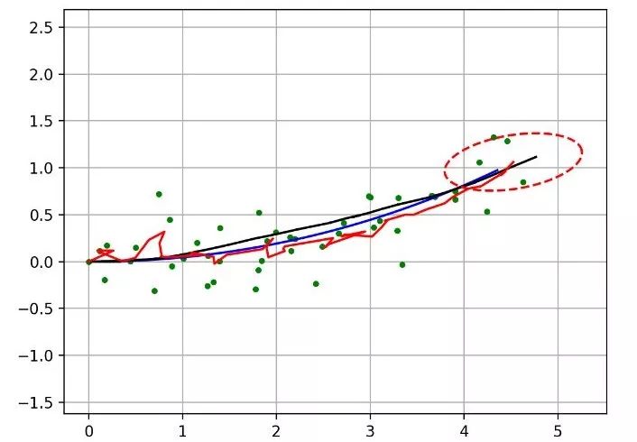
This algorithm uses the Extended Kalman Filter (EKF) for sensor fusion localization.

The blue line represents the true path, the black line indicates the dead reckoning trajectory, the green dots are position observations (like GPS), and the red line is the path estimated by EKF.

The red ellipse shows the covariance estimated by EKF.

Related Reading:

Probabilistic Robotics

http://www.probabilistic-robotics.org/

3.2 Unscented Kalman Filter Localization

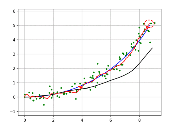
This algorithm utilizes the Unscented Kalman Filter (UKF) for sensor fusion localization.

The meanings of the lines and points are the same as in the EKF simulation example.

Related Reading:

Robot Localization Using Discriminatively Trained Unscented Kalman Filter

https://www.researchgate.net/publication/267963417_Discriminatively_Trained_Unscented_Kalman_Filter_for_Mobile_Robot_Localization

3.3 Particle Filter Localization

This algorithm uses the Particle Filter (PF) for sensor fusion localization.

The blue line represents the true path, the black line indicates the dead reckoning trajectory, the green dots are position observations (like GPS), and the red line is the path estimated by PF.

This algorithm assumes that the robot can measure the distance to landmarks (RFID).

PF localization will utilize these measurements.

Related Reading:

Probabilistic Robotics

http://www.probabilistic-robotics.org/

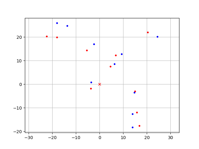
3.4 Histogram Filter Localization

This algorithm demonstrates 2D localization using a Histogram Filter.

The red cross represents the actual position, the black dot indicates the RFID position.

The blue grid shows the probability location from the Histogram Filter.

In this simulation, x and y are unknown, while yaw is known.

The filter integrates velocity input and distance observations obtained from RFID for localization.

No initial position is required.

Related Reading:

Probabilistic Robotics

http://www.probabilistic-robotics.org/

4. Mapping

4.1 Gaussian Grid Mapping

This algorithm demonstrates 2D Gaussian grid mapping.

4.2 Ray Casting Grid Mapping

This algorithm demonstrates 2D ray casting grid mapping.

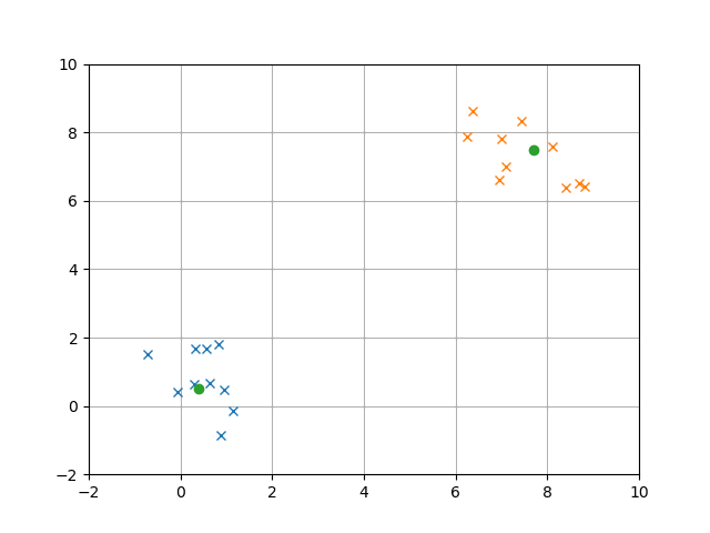
4.3 K-means Object Clustering

This algorithm demonstrates 2D object clustering using the K-means algorithm.

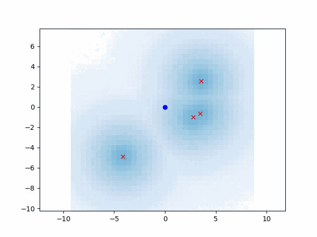
4.4 Circle Fitting Object Shape Recognition

This algorithm demonstrates object shape recognition using circle fitting.

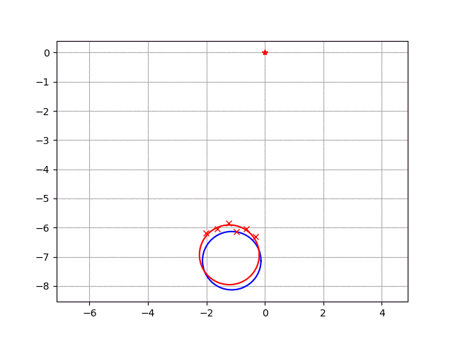
The blue circle represents the actual object shape.

The red cross indicates the points observed by the distance sensor.

The red circle is the estimated object shape using circle fitting.

5. SLAM

This section includes examples of Simultaneous Localization and Mapping (SLAM).

5.1 Iterative Closest Point Matching

This algorithm shows 2D Iterative Closest Point (ICP) matching using Singular Value Decomposition.

It calculates the rotation matrix and translation matrix from some points to others.

Related Reading:

Introduction to Robot Motion: Iterative Closest Point Algorithm

https://cs.gmu.edu/~kosecka/cs685/cs685-icp.pdf

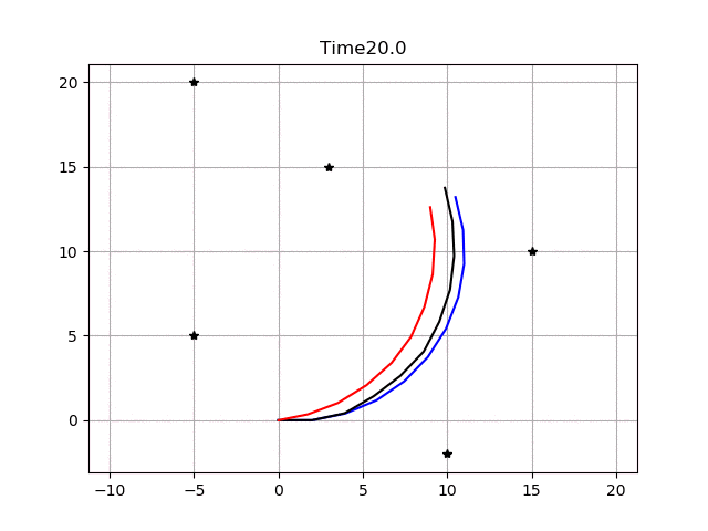
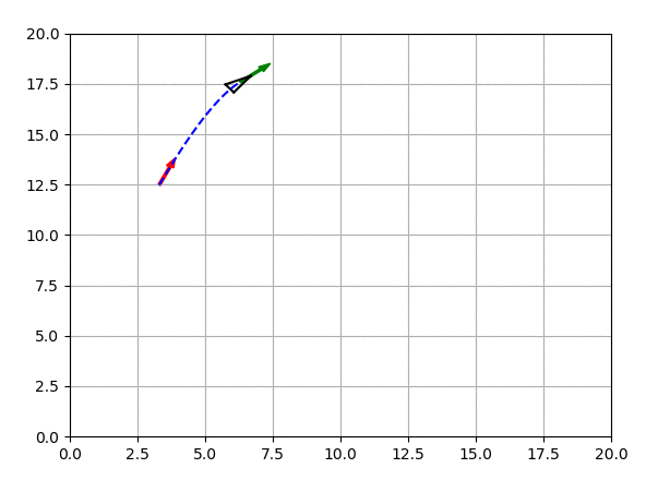
5.2 EKF SLAM

This is an example of SLAM based on the Extended Kalman Filter.

The blue line represents the true path, the black line indicates the dead reckoning trajectory, and the red line is the path estimated by EKF SLAM.

The green cross indicates the estimated landmarks.

Related Reading:

Probabilistic Robotics

http://www.probabilistic-robotics.org/

5.3 FastSLAM 1.0

This is an example of feature-based SLAM using FastSLAM 1.0.

The blue line represents the actual path, the black line indicates the dead reckoning, and the red line is the path estimated by FastSLAM.

The red dots are the particles in FastSLAM.

The black dots are the landmarks, and the blue crosses are the estimated landmark positions in FastSLAM.

Related Reading:

Probabilistic Robotics

http://www.probabilistic-robotics.org/

5.4 FastSLAM 2.0

This is an example of feature-based SLAM using FastSLAM 2.0.

The animation’s meaning is the same as in the case of FastSLAM 1.0.

Related Reading:

Probabilistic Robotics

http://www.probabilistic-robotics.org/

Tim Bailey’s SLAM Simulations

http://www-personal.acfr.usyd.edu.au/tbailey/software/slam_simulations.htm

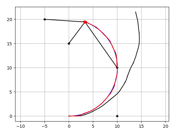
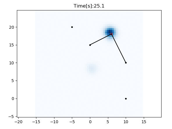
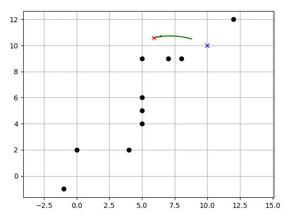
5.5 Graph-based SLAM

This is an example of graph-based SLAM.

The blue line represents the actual path.

The black line indicates the navigation estimate path.

The red line is the path estimated by graph-based SLAM.

The black stars are landmarks used to generate edges in the graph.

Related Reading:

Introduction to Graph-based SLAM

http://www2.informatik.uni-freiburg.de/~stachnis/pdf/grisetti10titsmag.pdf

6. Path Planning

6.1 Dynamic Window Approach

This is an example code for 2D navigation using the Dynamic Window Approach.

Related Reading:

Avoiding Collisions with the Dynamic Window Approach

https://www.ri.cmu.edu/pub_files/pub1/fox_dieter_1997_1/fox_dieter_1997_1.pdf

6.2 Grid-based Search

• Dijkstra’s Algorithm

This is grid-based shortest path planning using Dijkstra’s algorithm.

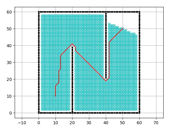
The cyan points in the animation represent the nodes that have been searched.

• A* Algorithm

This is grid-based shortest path planning using the A* algorithm.

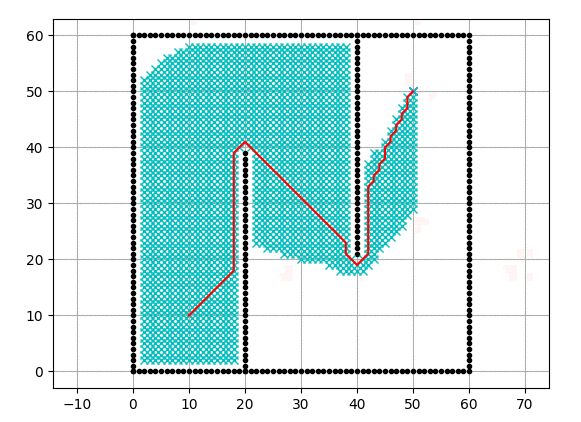
The cyan points in the animation represent the nodes that have been searched.

The heuristic used is the Euclidean distance in 2D.

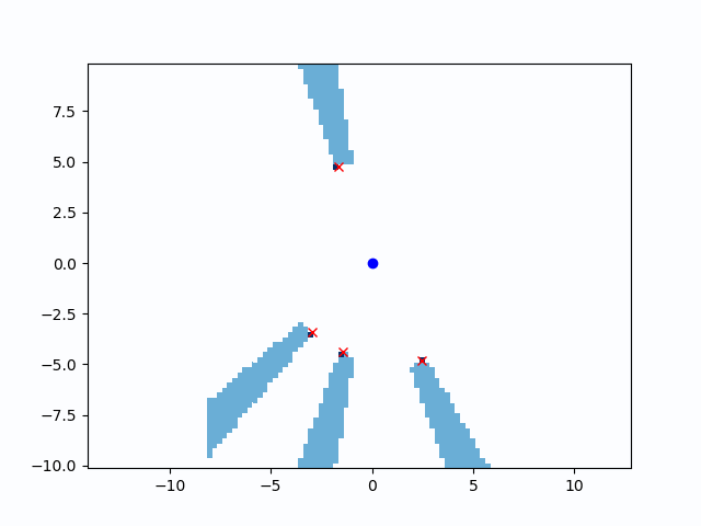
• Potential Field Algorithm

This demonstrates path planning using the Potential Field Algorithm.

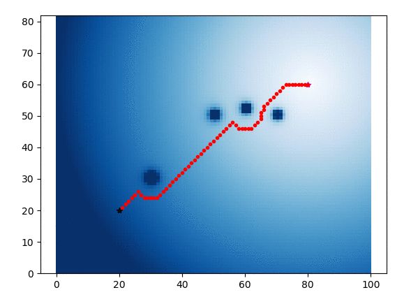
The blue heat map in the animation shows the potential energy of each grid.

Related Reading:

Robot Motion Planning: Potential Functions

https://www.cs.cmu.edu/~motionplanning/lecture/Chap4-Potential-Field_howie.pdf

6.3 Model Predictive Path Generation

This is a path optimization example for model predictive path generation.

The algorithm is used for state lattice planning.

• Path Optimization Example

• Lookup Table Generation Example

Related Reading:

Optimal Rough Terrain Path Generation for Wheeled Robots

http://journals.sagepub.com/doi/pdf/10.1177/0278364906075328

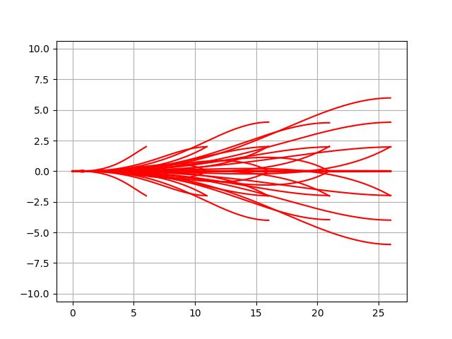
6.4 State Lattice Planning

This script uses state lattice planning to implement path planning.

This code addresses boundary issues through model predictive path generation.

Related Reading:

Optimal Rough Terrain Path Generation for Wheeled Robots

http://journals.sagepub.com/doi/pdf/10.1177/0278364906075328

Feasible Motion Sampling in High-Performance Mobile Robot Navigation in Complex Environments

http://www.frc.ri.cmu.edu/~alonzo/pubs/papers/JFR_08_SS_Sampling.pdf

• Uniform Polar Sampling (Uniform Polar Sampling)

• Biased Polar Sampling

• Lane Sampling

6.5 Probabilistic Roadmap (PRM) Planning

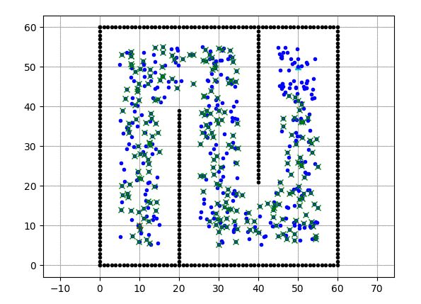
This Probabilistic Roadmap (PRM) planning algorithm uses Dijkstra’s method for graph search.

The blue points in the animation are the sampled points.

The cyan crosses represent the points searched by Dijkstra’s method.

The red line indicates the final path of PRM.

Related Reading:

Probabilistic Roadmap

https://en.wikipedia.org/wiki/Probabilistic_roadmap

6.6 Voronoi Path Planning

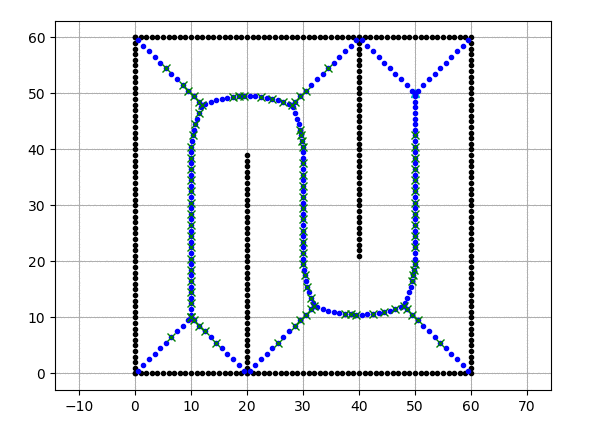
This Voronoi path planning algorithm uses Dijkstra’s method for graph search.

The blue points in the animation represent the Voronoi points.

The cyan crosses indicate the points searched by Dijkstra’s method.

The red line indicates the final path of the Voronoi path planning.

Related Reading:

Robot Motion Planning

https://www.cs.cmu.edu/~motionplanning/lecture/Chap5-RoadMap-Methods_howie.pdf

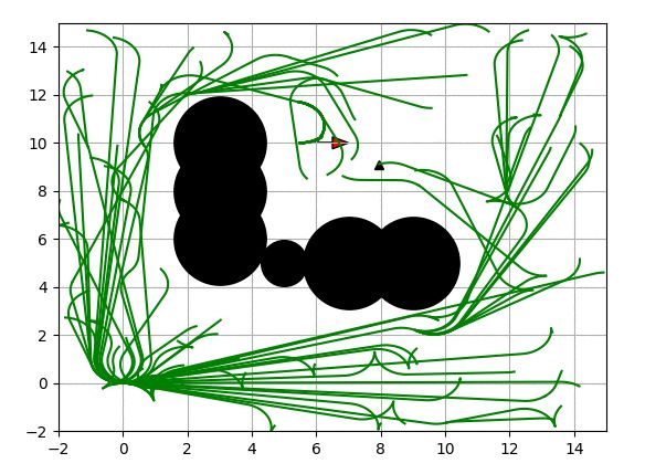
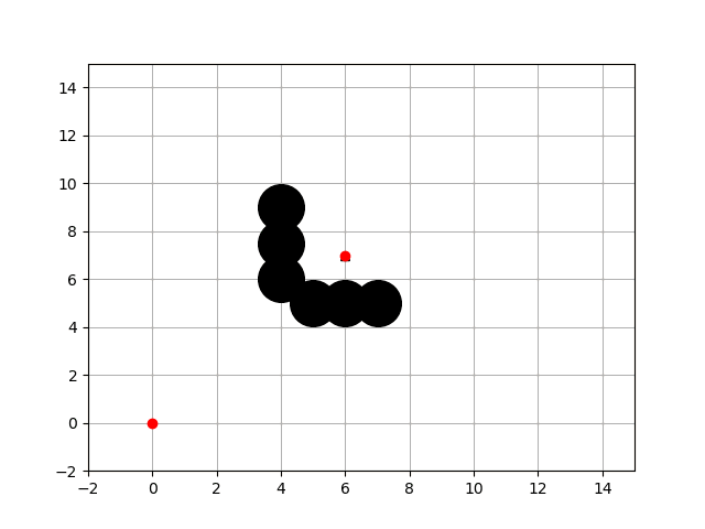
6.7 Rapidly-exploring Random Trees (RRT)

• Basic RRT

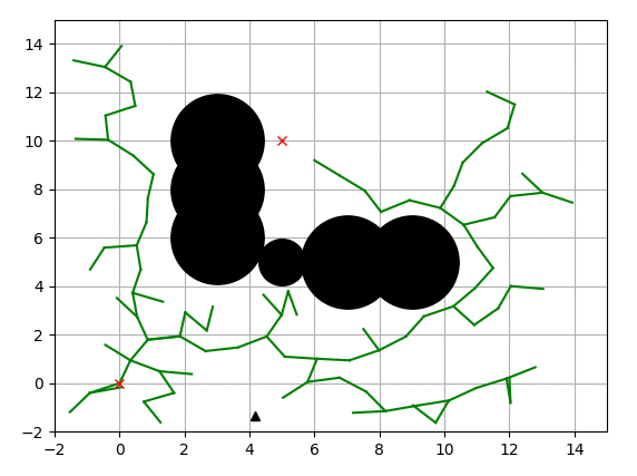
This is a simple path planning code using Rapidly-exploring Random Trees (RRT).

The black circles are obstacles, the green lines represent the search tree, and the red crosses indicate the start and goal positions.

• RRT*

This is a path planning code using RRT*.

The black circles are obstacles, the green lines represent the search tree, and the red crosses indicate the start and goal positions.

Related Reading:

Incremental Sampling-based Algorithms for Optimal Motion Planning

https://arxiv.org/abs/1005.0416

Sampling-based Algorithms for Optimal Motion Planning

http://citeseerx.ist.psu.edu/viewdoc/download?doi=10.1.1.419.5503&rep=rep1&type=pdf

• Dubins Path-based RRT

This path planning algorithm uses RRT and Dubins path for car-like robots.

• Dubins Path-based RRT*

This path planning algorithm uses RRT* and Dubins path for car-like robots.

• Reeds-Shepp Path-based RRT*

This path planning algorithm uses RRT* and Reeds-Shepp path for car-like robots.

• Informed RRT*

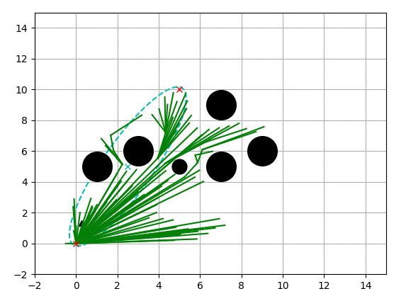
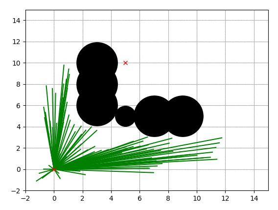
This is a path planning code using Informed RRT*.

The cyan ellipse indicates the sampling domain for Informed RRT*.

Related Reading:

Informed RRT*: Optimal Sampling-based Motion Planning via Direct Sampling of Acceptable Ellipsoids

https://arxiv.org/pdf/1404.2334.pdf

• Batch Informed RRT*

This is a path planning code using Batch Informed RRT*.

Related Reading:

Batch Informed Trees (BIT*): Optimal Planning via Heuristic Search on Implicit Random Geometric Graphs

https://arxiv.org/abs/1405.5848

• Closed Loop RRT*

This is a path planning algorithm using Closed Loop RRT* based on vehicle models.

In this code, steering control uses the pure pursuit algorithm.

Speed control uses PID.

Related Reading:

Motion Planning in Complex Environments Using Closed Loop Prediction

http://acl.mit.edu/papers/KuwataGNC08.pdf)

Real-time Motion Planning for Autonomous Urban Driving

http://acl.mit.edu/papers/KuwataTCST09.pdf

[1601.06326] Sampling-based Algorithms for Optimal Motion Planning Using Closed Loop Prediction

https://arxiv.org/abs/1601.06326

• LQR-RRT*

This is a simulation using LQR-RRT* for path planning.

LQR local planning uses a double integrator motion model.

Related Reading:

LQR-RRT*: Optimal Sampling-based Motion Planning via Automatic Differentiation of the Extended Heuristic

http://lis.csail.mit.edu/pubs/perez-icra12.pdf

MahanFathi/LQR-RRTstar: LQR-RRT* Method for Stochastic Motion Planning in the Pendulum Phase

https://github.com/MahanFathi/LQR-RRTstar

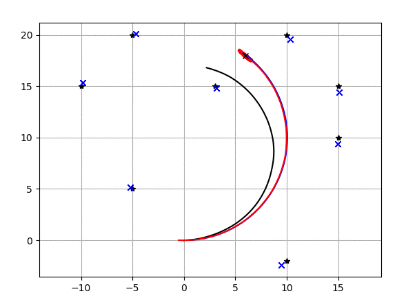
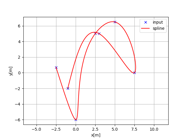
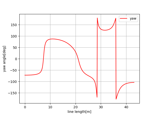
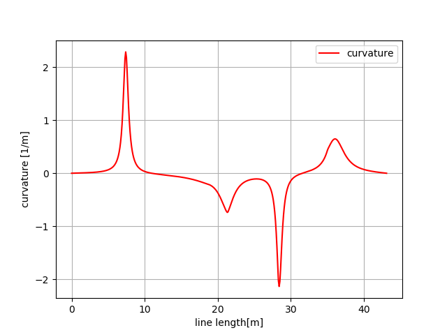
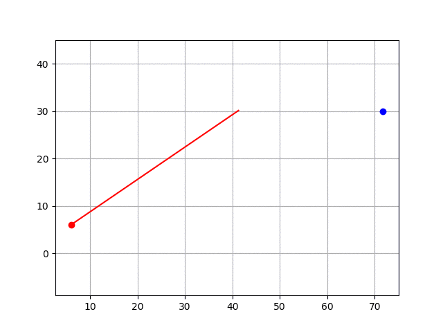
6.8 Cubic Spline Planning

This is an example code for cubic path planning.

This code generates a curvature continuous path based on x-y waypoints using cubic splines.

The direction angle of each point can also be calculated analytically.

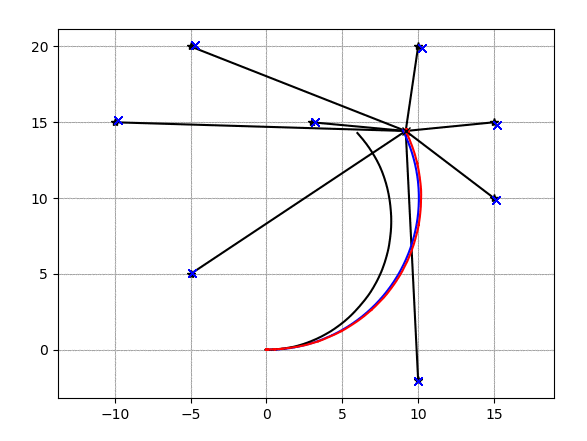
6.9 B-spline Planning

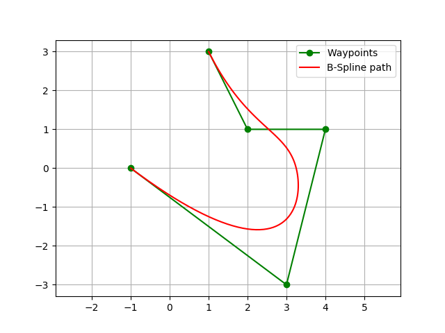
This is an example of planning using B-spline curves.

Input waypoints, and it will generate a smooth path using B-splines.

The first and last waypoints are located on the final path.

Related Reading:

B-splines

https://en.wikipedia.org/wiki/B-spline

6.10 Eta^3 Spline Path Planning

This is path planning using Eta^3 spline curves.

Related Reading:

η^3-Splines for the Smooth Path Generation of Wheeled Mobile Robots

https://ieeexplore.ieee.org/document/4339545/

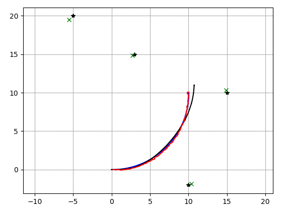
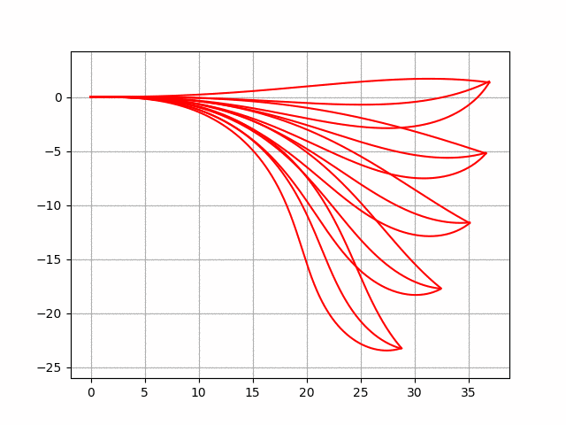
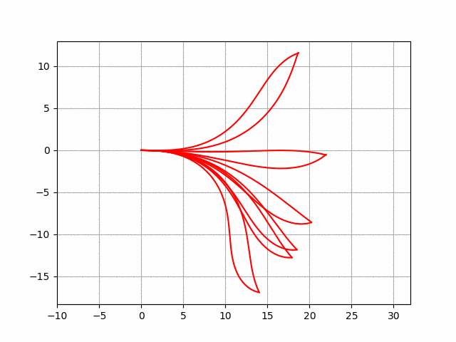
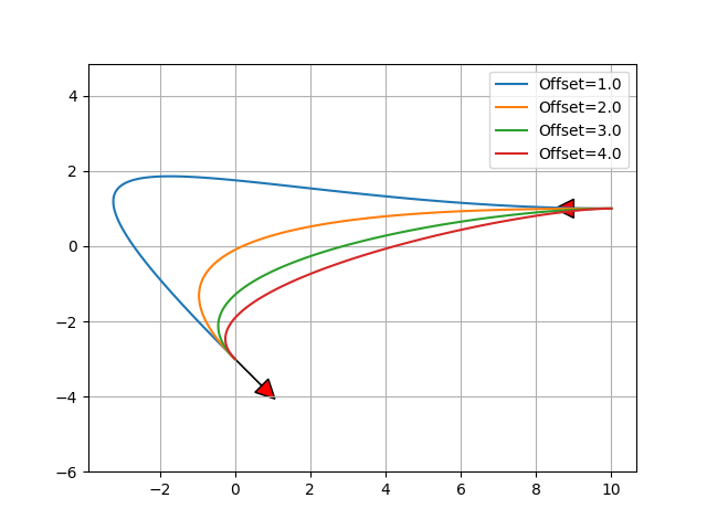
6.11 Bezier Path Planning

This is an example code for Bezier path planning.

Generates Bezier paths based on four control points.

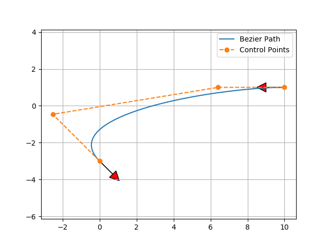
Changing the offset distance of the start and end points can generate different Bezier paths:

Related Reading:

Generating Curvature Continuous Paths for Autonomous Vehicles Based on Bezier Curves

http://citeseerx.ist.psu.edu/viewdoc/download?doi=10.1.1.294.6438&rep=rep1&type=pdf

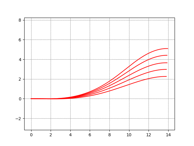
6.12 Quintic Polynomial Planning

Path planning using quintic polynomials.

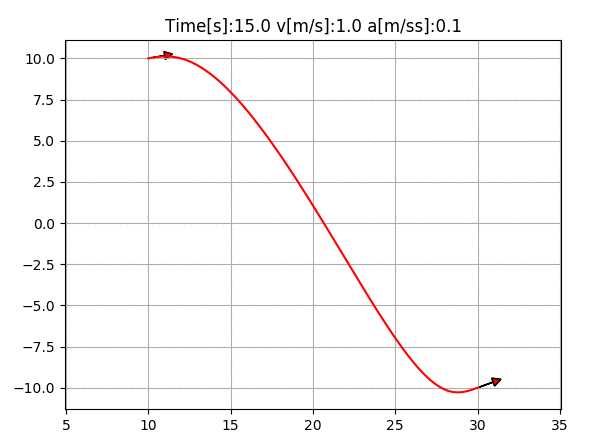
It can calculate 2D paths, velocity, and acceleration based on quintic polynomials.

Related Reading:

Local Path Planning and Motion Control for AGV In Positioning

http://ieeexplore.ieee.org/document/637936/

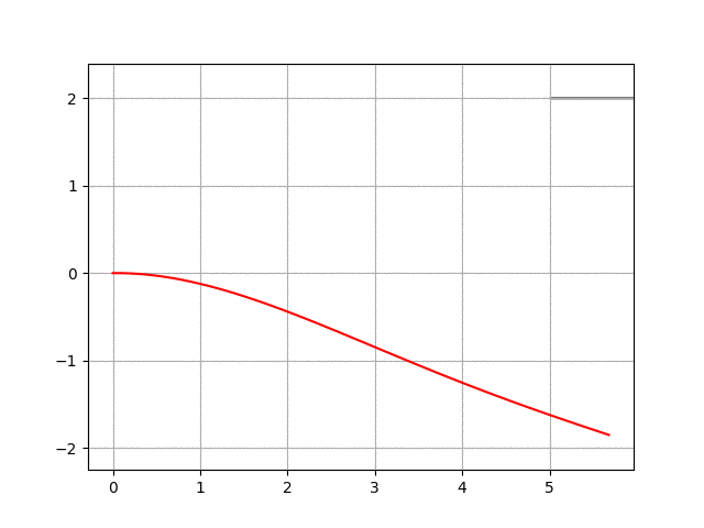
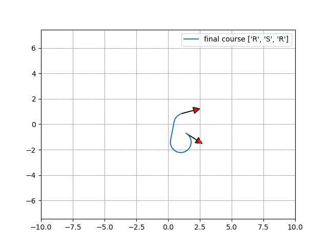
6.13 Dubins Path Planning

This is an example code for Dubins path planning.

Related Reading:

Dubins Path

https://en.wikipedia.org/wiki/Dubins_path

6.14 Reeds Shepp Path Planning

This is an example code for Reeds Shepp path planning.

Related Reading:

15.3.2 Reeds-Shepp Curves

http://planning.cs.uiuc.edu/node822.html

Optimal Paths for Cars that Can Go Forward and Backward

https://pdfs.semanticscholar.org/932e/c495b1d0018fd59dee12a0bf74434fac7af4.pdf

ghliu/pyReedsShepp: Implementing Reeds Shepp Curves

https://github.com/ghliu/pyReedsShepp

6.15 Path Planning Based on LQR

This is an example code for path planning using LQR for a double integrator model.

6.16 Optimal Path in Frenet Frame

This code generates the optimal path in the Frenet Frame.

The cyan line represents the target path, the black cross represents obstacles.

The red line represents the predicted path.

Related Reading:

Optimal Path Generation in Dynamic Scenes in a Frenet Frame

https://www.researchgate.net/profile/Moritz_Werling/publication/224156269_Optimal_Trajectory_Generation_for_Dynamic_Street_Scenarios_in_a_Frenet_Frame/links/54f749df0cf210398e9277af.pdf

Optimal Path Generation in Dynamic Scenes in a Frenet Frame

https://www.youtube.com/watch?v=Cj6tAQe7UCY

7. Path Tracking

7.1 Pose Control Tracking

This is a simulation of pose control tracking.

Related Reading:

Robotics, Vision and Control – Fundamental Algorithms In MATLAB® Second, Completely Revised, Extended And Updated Edition | Peter Corke | Springer

https://www.springer.com/us/book/9783319544120

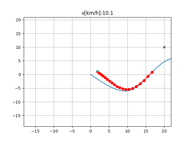
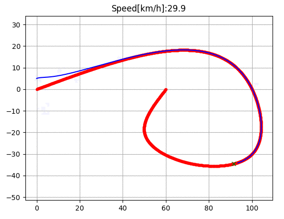
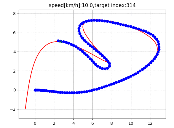
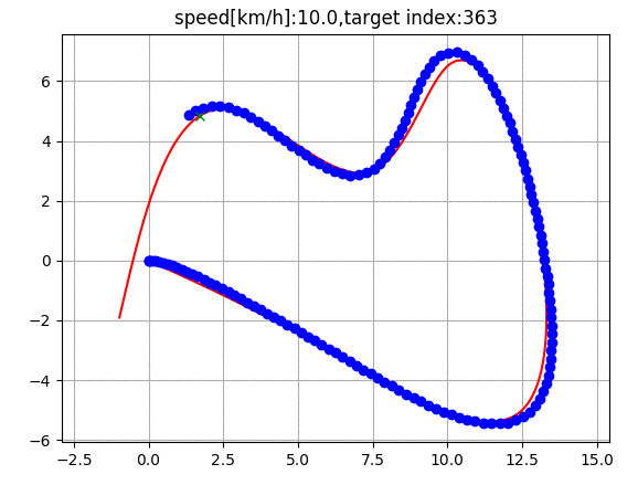
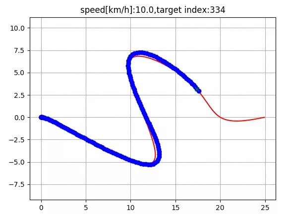
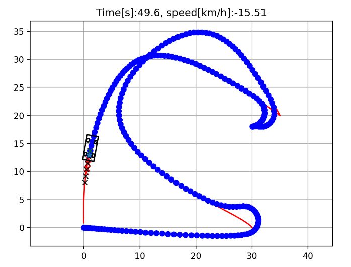
7.2 Pure Pursuit Tracking

This is a path tracking simulation using pure pursuit steering control and PID speed control.

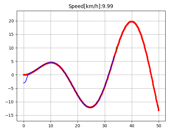
The red line represents the target route, the green cross indicates the target point of pure pursuit control, and the blue line shows the tracking route.

Related Reading:

Survey on Motion Planning and Control Techniques for Autonomous Vehicles in Urban Environments

https://arxiv.org/abs/1604.07446

7.3 Stanley Control

This is a path tracking simulation using Stanley steering control and PID speed control.

Related Reading:

Stanley: The Robot That Won the DARPA Grand Challenge

http://robots.stanford.edu/papers/thrun.stanley05.pdf

Automatic Steering Methods for Path Tracking of Autonomous Vehicles

https://www.ri.cmu.edu/pub_files/2009/2/Automatic_Steering_Methods_for_Autonomous_Automobile_Path_Tracking.pdf

7.4 Rear Wheel Feedback Control

This is a path tracking simulation using rear wheel feedback steering control and PID speed control.

Related Reading:

Survey on Motion Planning and Control Techniques for Autonomous Vehicles in Urban Environments

https://arxiv.org/abs/1604.07446

7.5 Linear Quadratic Regulator (LQR) Steering Control

This is a path tracking simulation using LQR steering control and PID speed control.

Related Reading:

ApolloAuto/apollo: Open Source Autonomous Driving Platform

https://github.com/ApolloAuto/apollo

7.6 Linear Quadratic Regulator (LQR) Steering and Speed Control

This is a path tracking simulation using LQR steering and speed control.

Related Reading:

Fully Autonomous Driving: Systems and Algorithms – IEEE Conference Publications

http://ieeexplore.ieee.org/document/5940562/

7.7 Model Predictive Speed and Steering Control

This is a path tracking simulation using iterative linear model predictive speed and steering control.

This code uses cxvxpy as the optimal modeling tool.

Related Reading:

Vehicle Dynamics and Control | Rajesh Rajamani | Springer

http://www.springer.com/us/book/9781461414322

MPC Course Material – MPC Lab @ UC-Berkeley

http://www.mpc.berkeley.edu/mpc-course-material

8. Project Support

You can financially support this project through Patreon (https://www.patreon.com/myenigma).

If you support this project on Patreon, you will receive email technical support regarding the project’s code.

The authors of this article include Atsushi Sakai (@Atsushi_twi), Daniel Ingram, Joe Dinius, Karan Chawla, Antonin RAFFIN, Alexis Paques.

Original text:

https://atsushisakai.github.io/PythonRobotics/#what-is-this

Author:Atsushi Sakai, a Japanese robotics engineer engaged in autonomous driving technology development, proficient in C++, ROS, MATLAB, Python, Vim, and Robotics.

Translator:Wanyue, Editor: Guo Rui

Good news!
Beginner's Visual Learning Knowledge Community
Is now open to the public 👇👇👇



Download 1: OpenCV-Contrib Extension Module Chinese Version Tutorial
Reply "Extension Module Chinese Tutorial" in the "Beginner's Visual Learning" public account backend to download the first Chinese version of OpenCV extension module tutorial on the internet, covering more than twenty chapters including extension module installation, SFM algorithms, stereo vision, object tracking, biological vision, super-resolution processing, etc.

Download 2: 52 Lectures on Python Vision Practical Projects
Reply "Python Vision Practical Projects" in the "Beginner's Visual Learning" public account backend to download 31 visual practical projects including image segmentation, mask detection, lane detection, vehicle counting, adding eyeliner, license plate recognition, character recognition, emotion detection, text content extraction, face recognition, etc., to help quickly learn computer vision.

Download 3: 20 Lectures on OpenCV Practical Projects
Reply "20 Lectures on OpenCV Practical Projects" in the "Beginner's Visual Learning" public account backend to download 20 practical projects based on OpenCV to advance OpenCV learning.

Discussion Group

You are welcome to join the public account reader group to communicate with peers. Currently, there are WeChat groups for SLAM, 3D vision, sensors, autonomous driving, computational photography, detection, segmentation, recognition, medical imaging, GAN, algorithm competitions, etc. (will gradually be subdivided in the future). Please scan the WeChat number below to join the group, note: "Nickname + School/Company + Research Direction", for example: "Zhang San + Shanghai Jiao Tong University + Visual SLAM". Please follow the format for notes, otherwise, you will not be approved. After successful addition, you will be invited to join the relevant WeChat group based on research direction. Please do not send advertisements in the group, otherwise, you will be removed from the group. Thank you for your understanding~