[Introduction] Ah, you have been successfully drawn in, not quite what you expected, huh?~~~

Just kidding, back to the point. Today, a netizen asked me a question about a sensor measuring a physical quantity and needing to determine its trend of change. I provided some suggestions, and here I will elaborate on those suggestions and share them with everyone.

This article aims to express a personal viewpoint: when faced with unsolvable problems in development, one can try to approach the issue from a mathematical perspective to see if an answer can be found.

Note: The images in this article are just to make reading easier. My math skills are also mediocre, so please correct any mistakes.

What is the Pitfall?

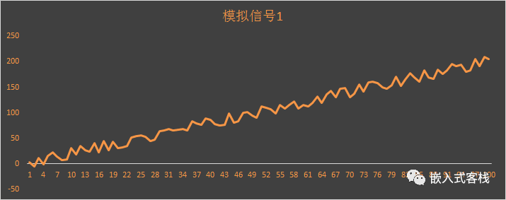
A sensor is used in a project to measure a physical quantity; let’s assume it measures temperature. We need to determine its trend of change and use this trend for some applications.

So how do we determine the trend of change for a physical quantity? Naturally, we might think of calculating the rate of change of this random sequence. This involves some definitions of sequences. Random sequences can have many possible sources, the most common being modulus sampling.

This converts the S(t) signal into a discrete signal sequence S(n). So how do we calculate the slope at the current moment? (Here we ignore the intermediate transitional states and only consider it as connected line segments; of course, in real applications, if there are higher requirements, curve fitting can be done.)

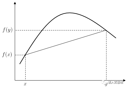
However, simply judging the slope can easily lead to misjudgment, as in the following situation:

The slope alternates between positive and negative, but the overall trend is increasing. Therefore, examining only the slope is clearly not advisable; the code needs to add various complex conditions or limits for judgment. Even with so many conditions, the system may still perform very unreliably.

For the analog signal 2, the trend is constantly changing. So how can we stabilize it? Should I keep you in suspense?

Concavity and Convexity of Functions

Concave Functions

A concave function is a real-valued function f defined on a convex set C (interval) in some vector space. Let f be a function defined on interval I. If for any two points x1<x2 in I and any real number t belonging to (0,1), it holds that

then the function f is called a concave function on I, which some books also refer to as a lower convex function.

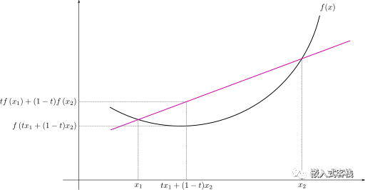
If we change the “≥” in the above condition to “>”, it is called a strictly concave function or strictly lower convex function.

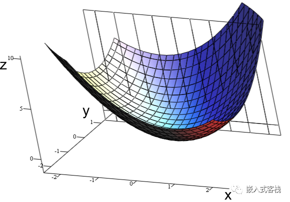
The above is the case for one-dimensional functions; here is a graph for two-dimensional functions for easier understanding.

Convex Functions

Let f be a function defined on interval I. If for any two points x1<x2 in I and any real number t belonging to (0,1), the above inequality becomes greater than or equal to, then it is a convex function on that interval.

It can be seen that concavity and convexity are relative; for example, if f(x) is concave in a certain interval, then -f(x) is convex in that interval.

Properties

• If a function is twice differentiable in a certain interval and the second derivative is greater than 0, then the function is concave in that interval.
• If a function is twice differentiable in a certain interval and the second derivative is less than 0, then the function is convex in that interval.

Proof: I won’t derive it here, but you can use the Mean Value Theorem to derive the above property.

Let’s take a look at a dynamic graph to deepen our understanding:

The function’s tangent line is shown in blue, the curve is concave upwards, green indicates the curve is concave downwards, and red indicates the inflection point of the curve.

The first derivative of sin(2x) is:

The second derivative of sin(2x) is:

End of the show, though I might not have shown it correctly~~~

Back to the Pitfall

Through the previous show-off, can we use the derivative of discrete sequences to determine the trend of change of the sensor? What? Derivative? Are we going to start showing off again?

Earlier, we said the first derivative is like this:

So what does the second derivative look like?

Let’s simplify it:

Where S[n] represents the current measurement point, S[n-1] represents the previous measurement point, and S[n-2] represents the second previous measurement point. It should be +S[n-2]

Let’s Code

#include <stdio.h>
#include <math.h>
#include <string.h>
typedef struct _T_2ND_DRV
{
    float xn1;
    float xn2;
}t_2ND_DRV;
typedef struct _T_1ST_DRV
{
    float xn1;
}t_1ST_DRV;

void init_second_derivative(t_2ND_DRV *pSndDrv)
{
    pSndDrv->xn1 = 0;
    pSndDrv->xn2 = 0;
}

float second_derivative(t_2ND_DRV *pSndDrv, float xn,float T)
{
     float result=0.0f;
     if(T<=0)
         return 0x7FBFFFFF; /*非法数据*/
     result = (xn-2*pSndDrv->xn1+pSndDrv->xn2)/T/T;
     pSndDrv->xn2 = pSndDrv->xn1;
     pSndDrv->xn1 = xn;
    
     return result;
}

void init_fisrt_derivative(t_1ST_DRV *p1stDrv)
{
    p1stDrv->xn1 = 0;
}

float fisrt_derivative(t_1ST_DRV *p1stDrv, float xn,float T)
{
     float result=0.0f;
     if(T<=0)
         return 0x7FBFFFFF; /*非法数据*/
     result = (xn-p1stDrv->xn1)/T; 
     p1stDrv->xn1 = xn;
    
     return result;
}
#define PI 3.1415f
#define SAMPLE_RATE 500.0f
#define SAMPLE_T (1/SAMPLE_RATE)
#define SAMPLE_SIZE (100)
int main()
{
    float sim1[SAMPLE_SIZE];
    float sim2[SAMPLE_SIZE];
    float out1[SAMPLE_SIZE];
    float out2[SAMPLE_SIZE];
    t_2ND_DRV sndDrv;
    t_1ST_DRV frtDrv;
    init_fisrt_derivative(&frtDrv);
    init_second_derivative(&sndDrv);
    
    FILE *pFile=fopen("./simulationSin.csv","wt+");
    if(pFile==NULL)
    {
        printf("simulationSin.csv opened failed");
        return -1;
    }
    
    for(int i=0;i<SAMPLE_SIZE;i++)
    {
        sim1[i]=10*sin(2*PI*10*i/500);
    } 
    for(int i=0;i<SAMPLE_SIZE;i++)
    {
        out1[i]=fisrt_derivative(&frtDrv,sim1[i],SAMPLE_T);
        out2[i]=second_derivative(&sndDrv,sim1[i],SAMPLE_T);
        fprintf(pFile,"%f,%f,%f\n",sim1[i],out1[i],out2[i]);
    }

    fclose(pFile);

    return 0;
}

Ignore the first two points and use Excel to generate the curve:

From the graph, we can see:

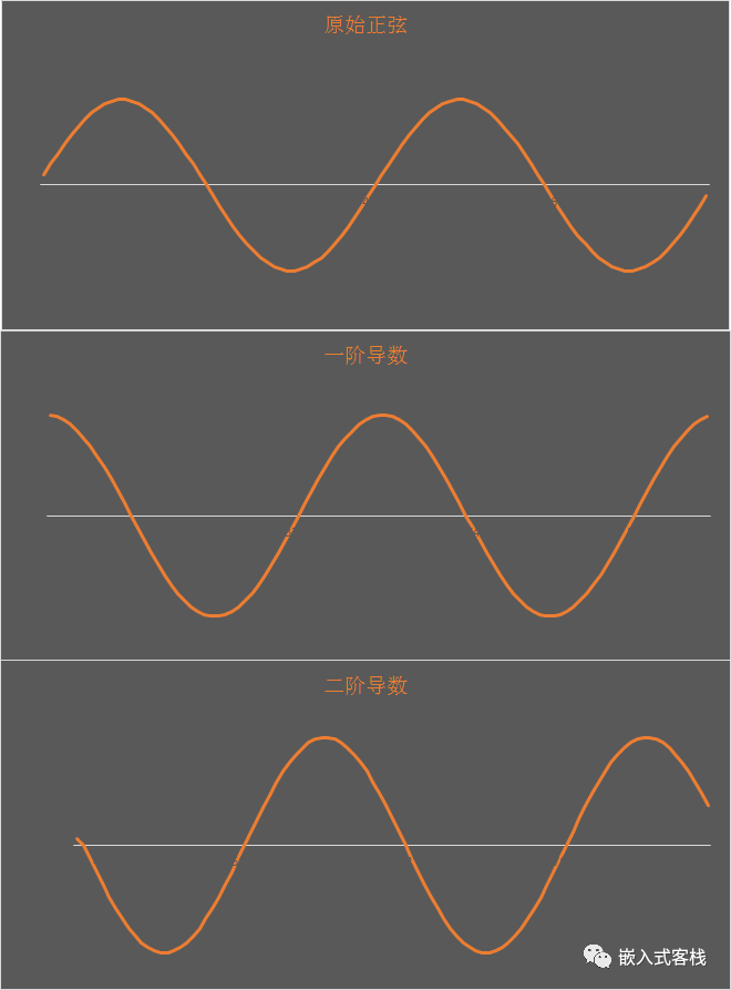
• When the first derivative is positive, the function is increasing;
• When the first derivative is negative, the function is decreasing;
• When the second derivative is 0, an inflection point occurs, and the trend changes; if the signs of the first derivatives on both sides are opposite, an extremum occurs.
• When the second derivative is negative, the first derivative, i.e., the slope of the original function, decreases monotonically; when the second derivative is positive, the first derivative increases monotonically.

Further:

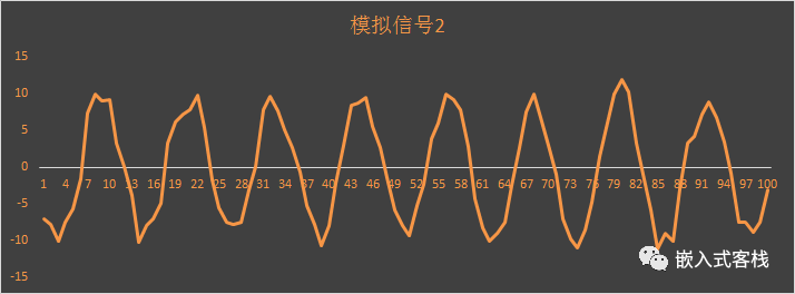
By looking at the first and second derivatives together, we can see the trend of change in the measured values. For example, in the first quarter of the cycle, the trend is increasing, meaning the first derivative is positive, while the second derivative is negative, indicating that the increasing trend is gradually decreasing to 0.

Code Optimization

If we are only making qualitative judgments, the above functions do not need to divide by the sampling period; we can simply examine the increments. The code can be optimized as follows:

typedef struct _T_2ND_DRV
{
    float xn1;
    float xn2;
}t_2ND_DRV;
typedef struct _T_1ST_DRV
{
    float xn1;
}t_1ST_DRV;

void init_second_derivative(t_2ND_DRV *pSndDrv)
{
    pSndDrv->xn1 = 0;
    pSndDrv->xn2 = 0;
}

float second_derivative(t_2ND_DRV *pSndDrv, float xn)
{
     float result=0.0f;
     result = xn-2*pSndDrv->xn1+pSndDrv->xn2;
     pSndDrv->xn2 = pSndDrv->xn1;
     pSndDrv->xn1 = xn;
    
     return result;
}

void init_fisrt_derivative(t_1ST_DRV *p1stDrv)
{
    p1stDrv->xn1 = 0;
}

float fisrt_derivative(t_1ST_DRV *p1stDrv, float xn)
{
     float result=0.0f;
     result = xn-p1stDrv->xn1; 
     p1stDrv->xn1 = xn;
    
     return result;
}

Unexpected Gains

Here, I unexpectedly introduce a knowledge point that many people may not have noticed: NaN. In calculations, NaN represents ‘Not a Number’, a member of numeric data types, which can be interpreted as an uncertain or unrepresentable value, especially in floating-point operations. In 1985, the IEEE 754 floating-point standard introduced NaN for system use and represented other infinite quantities (such as infinity).

The aforementioned function returns 0x7FBFFFFF, which represents infinity.

Different operating systems and programming languages may have different string representations of NaN:

nan
 NaN
 NaN%
 NAN
 NaNQ
 NaNS
 qNaN
 sNaN
 1.#SNAN
 1.#QNAN
 -1.#IND

In fact, since the encoded NaN has a sign, they can often also be found in the string representation of NaN, such as:

 -NaN
  NaN12345
 -sNaN12300
 -NaN(s1234)

Engineering Applications

Here is my suggested solution:

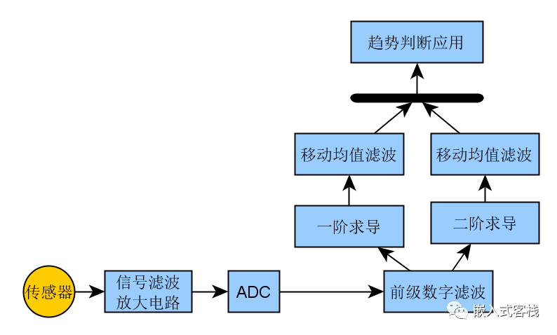
Process the sensor signal through a circuit, perform analog-to-digital sampling, and then enter a digital filter to remove unnecessary noise before performing first and second derivatives. For the first and second derivatives, apply a moving average filter, and finally, based on the description above, determine the trend of change. I believe this approach is quite robust. The actual length of the moving average filter should not be too long; otherwise, the response will be delayed, making it impossible to make real-time judgments on the sensor’s trend of change. Adding a subsequent moving average filter will eliminate the impact of random noise interference caused by fluctuating waveforms, making the system’s judgment more robust. The actual filter length needs to be tuned and optimized based on different scenarios. Alternatively, other IIR/FIR filter forms can also be implemented.

In Summary

As an embedded programmer, sometimes it is necessary to look at math books and understand the stories behind mathematical principles, as it may bring unexpected benefits.