Click the “Learn Algorithms in Five Minutes” above and choose the “Star” public account
Heavy content delivered first

Source: Juejin, Author: Ruheng
Link: https://juejin.im/post/6844903490595061767
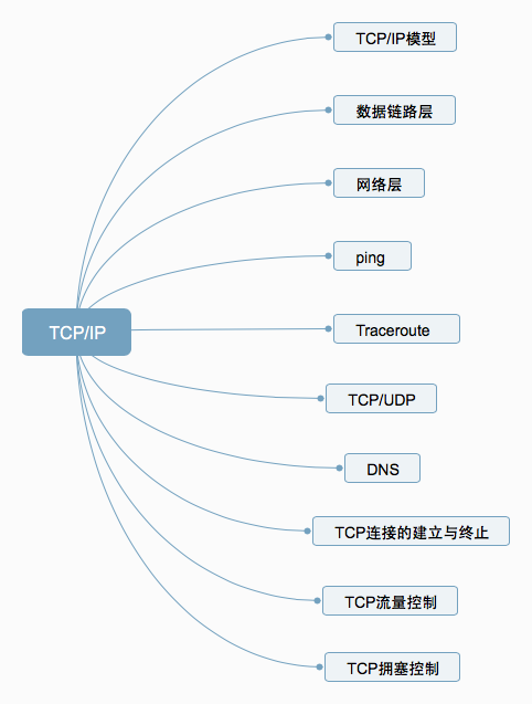
1. TCP/IP Model
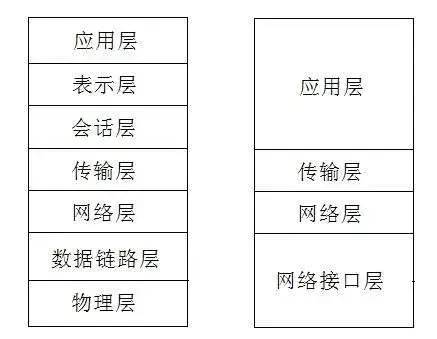
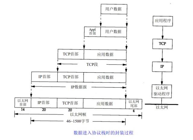
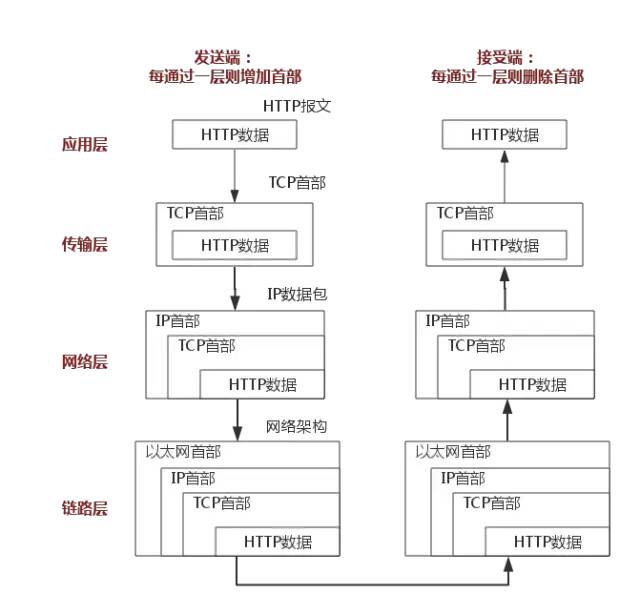
The above diagram uses the HTTP protocol as an example for a detailed explanation.
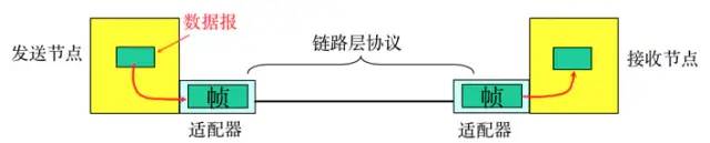
2. Data Link Layer
-
Encapsulating into frames: Add headers and trailers to the network layer datagram, encapsulating it into frames. The frame header includes the source MAC address and destination MAC address.
-
Transparent transmission: zero bit padding, escape characters.
-
Reliable transmission: Rarely used on low-error-rate links, but wireless links (WLAN) guarantee reliable transmission.
-
Error detection (CRC): The receiver detects errors, and if an error is found, the frame is discarded.
3. Network Layer
1. IP Protocol
The IP protocol is the core of the TCP/IP protocol, and all TCP, UDP, ICMP, IGMP data is transmitted in IP data format. It is important to note that IP is not a reliable protocol, meaning that the IP protocol does not provide a mechanism for handling data that has not been delivered, which is considered the responsibility of upper-layer protocols: TCP or UDP.
1.1 IP Address
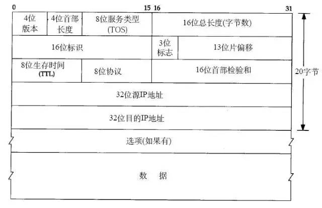
1.2 IP Protocol Header
2. ARP and RARP Protocols
3. ICMP Protocol
The IP protocol is not a reliable protocol; it does not guarantee data delivery. Therefore, the task of ensuring data delivery should naturally fall to other modules. One important module is the ICMP (Internet Control Message Protocol). ICMP is not a high-level protocol but is a protocol at the IP layer.
When errors occur in transmitting IP packets, such as host unreachable, route unreachable, etc., the ICMP protocol will encapsulate the error information and send it back to the host, giving the host a chance to handle the error. This is why protocols built on top of the IP layer can achieve reliability.
4. Ping
Ping can be said to be the most famous application of ICMP and is part of the TCP/IP protocol. The “ping” command can check network connectivity and is very helpful for analyzing and diagnosing network faults.
For example, when we cannot access a website, we usually ping the site. The ping will echo some useful information. General information is as follows:

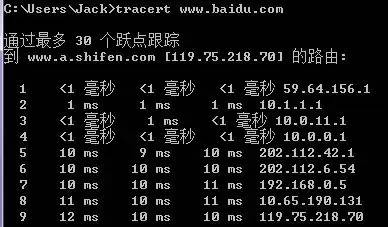
5. Traceroute
Traceroute is an important tool for detecting the routing situation between a host and the destination host, and it is the most convenient tool available.
The principle of Traceroute is quite interesting. Upon receiving the destination host’s IP, it first sends a UDP packet with TTL=1 to the destination host. The first router that receives this packet will automatically reduce the TTL by 1, and when the TTL becomes 0, the router discards the packet and generates an unreachable ICMP message back to the host. The host then sends a UDP packet with TTL=2 to the destination host, prompting the second router to send an ICMP message back to the host. This process continues until it reaches the destination host, allowing Traceroute to obtain all router IPs.
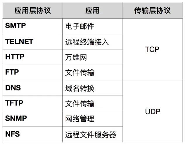
6. TCP/UDP

Message-oriented
The message-oriented transmission method allows the application layer to specify the length of the message to UDP, and UDP will send it as is, meaning one message per send. Therefore, the application must choose a suitable message size. If the message is too long, the IP layer needs to fragment it, reducing efficiency. If it is too short, it will be too small for IP.
Byte stream-oriented
When should TCP be used?
When should UDP be used?
7. DNS
8. Establishment and Termination of TCP Connections
1. Three-way Handshake
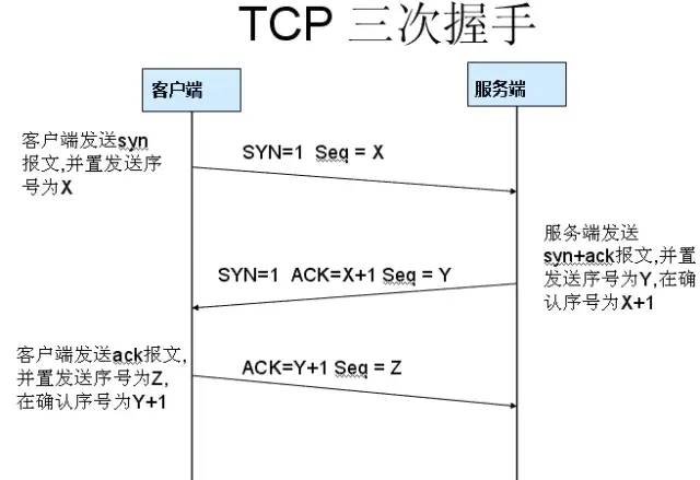
Why three-way handshake?
2. Four-way Handshake
After the client and server have established a TCP connection through the three-way handshake, when the data transmission is complete, the TCP connection must be terminated. This is known as the mysterious “four-way handshake”.
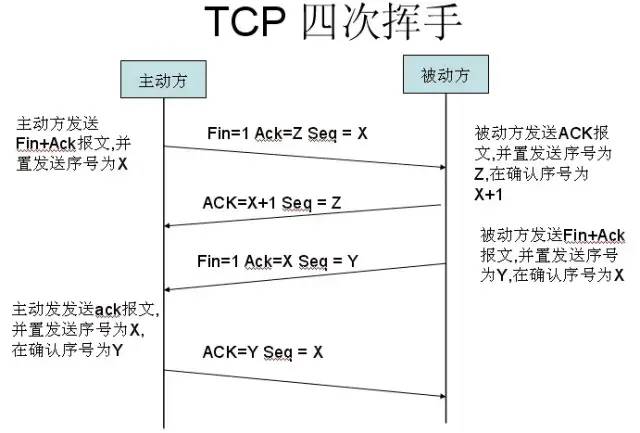
First separation: Host 1 (which can be either the client or server) sets the Sequence Number and sends a FIN segment to Host 2; at this point, Host 1 enters the FIN_WAIT_1 state; this indicates that Host 1 has no more data to send to Host 2;
Second separation: Host 2 receives the FIN segment from Host 1 and sends an ACK segment back to Host 1, with the Acknowledgment Number set to the Sequence Number plus 1; Host 1 enters the FIN_WAIT_2 state; Host 2 informs Host 1 that it “agrees” to the closure request;
Third separation: Host 2 sends a FIN segment to Host 1, requesting to close the connection, while Host 2 enters the LAST_ACK state;
Fourth separation: Host 1 receives the FIN segment from Host 2 and sends an ACK segment back to Host 2; then Host 1 enters the TIME_WAIT state; after Host 2 receives Host 1’s ACK segment, it closes the connection; at this point, Host 1 waits for 2MSL, and if it still has not received a reply, it can close the connection as well.
Why four-way handshake?
Why wait for 2MSL?
MSL: Maximum Segment Lifetime, which is the longest time any segment can exist in the network before being discarded. There are two reasons for this:
-
To ensure that the TCP protocol’s full-duplex connection can be reliably closed.
-
To ensure that any duplicate segments from this connection disappear from the network.
The first point: If Host 1 directly goes to CLOSED, and due to the unreliability of the IP protocol or other network reasons, Host 2 does not receive Host 1’s final ACK reply. Then Host 2 will continue to send FIN after a timeout. Since Host 1 has already CLOSED, it will not find the connection corresponding to the resent FIN. Therefore, Host 1 does not directly enter CLOSED, but maintains TIME_WAIT, so that when it receives FIN again, it can ensure that the other side receives the ACK, thereby correctly closing the connection.
The second point: If Host 1 directly goes to CLOSED and then initiates a new connection to Host 2, we cannot guarantee that the new connection will have a different port number than the recently closed connection. In other words, it is possible for the new connection and the old closed connection to have the same port number. Generally, this should not cause any problems, but there are special cases: If the new connection and the already closed old connection have the same port number, and some delayed data from the previous connection still lingers in the network, this delayed data will arrive at Host 2 after the new connection is established. Since the new connection and old connection have the same port number, the TCP protocol will mistakenly consider that delayed data belongs to the new connection, thus causing confusion with the actual data packets of the new connection. Therefore, the TCP connection must wait in the TIME_WAIT state for 2MSL to ensure that all data from the current connection disappears from the network.
9. TCP Flow Control
If the sender sends data too quickly, the receiver may not be able to keep up, leading to data loss. Flow control ensures that the sender’s sending rate is not too fast, allowing the receiver to keep up with the reception.
Using the sliding window mechanism makes it easy to implement flow control on a TCP connection.
Assume A is sending data to B. At the time of connection establishment, B informs A: “My receive window is rwnd = 400” (where rwnd represents the receiver window). Therefore, the sender’s sending window cannot exceed the value of the receiver window provided by the receiver. Note that the TCP window is measured in bytes, not segments. Assume each segment is 100 bytes long, and the initial value of the data segment sequence number is set to 1. Uppercase ACK indicates the acknowledgment bit in the header, while lowercase ack indicates the acknowledgment field value.

From the diagram, we can see that B performed flow control three times. The first time the window was reduced to rwnd = 300, the second time to rwnd = 100, and finally to rwnd = 0, which prohibits the sender from sending any more data. This state of pausing the sender will last until Host B sends a new window value.
TCP has a persistence timer for each connection. Whenever one side of the TCP connection receives a zero window notification from the other side, it starts the persistence timer. If the timer expires, it sends a zero-window probe segment (carrying 1 byte of data), and the party receiving this segment resets the persistence timer.
10. TCP Congestion Control
The sender maintains a congestion window (cwnd) state variable. The size of the congestion window depends on the network’s congestion level and changes dynamically. The sender sets its sending window equal to the congestion window.
The principle of controlling the congestion window is that as long as there is no congestion in the network, the congestion window increases to send more packets. However, whenever congestion occurs, the congestion window decreases to reduce the number of packets injected into the network.
The slow start algorithm:
When a host starts sending data, if it injects a large amount of data bytes into the network immediately, it may cause network congestion, as the load situation of the network is not clear. Therefore, a better method is to probe first, gradually increasing the sending window from small to large, meaning increasing the congestion window value gradually.
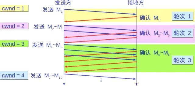
Typically, when starting to send packets, the congestion window cwnd is initially set to the value of one maximum segment size (MSS). After receiving an acknowledgment for a new segment, the congestion window is increased by at most one MSS. This gradual increase in the sender’s congestion window cwnd allows packets to be injected into the network at a more reasonable rate.
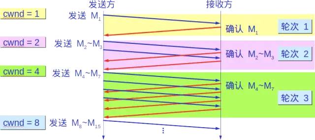
With each transmission round, the congestion window cwnd doubles. The time for one transmission round is actually the round-trip time RTT. However, “transmission round” emphasizes that all segments allowed to be sent by the congestion window cwnd are sent continuously, and the last byte sent receives acknowledgment.
Moreover, the “slow” in slow start does not refer to the slow growth rate of cwnd, but rather that during the initial sending of packets, cwnd is set to 1, allowing the sender to send only one segment initially (to probe the network’s congestion situation), and then gradually increases cwnd.
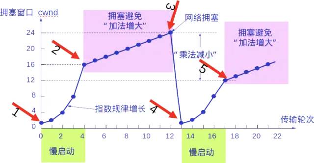
To prevent the congestion window cwnd from growing too large and causing network congestion, a slow start threshold (ssthresh) state variable is also set. The usage of the slow start threshold ssthresh is as follows:
-
When cwnd < ssthresh, use the above slow start algorithm.
-
When cwnd > ssthresh, stop using the slow start algorithm and switch to the congestion avoidance algorithm.
-
When cwnd = ssthresh, either the slow start algorithm or the congestion avoidance algorithm can be used.
Congestion avoidance
Slowly increase the congestion window cwnd, meaning that every round-trip time RTT, the sender’s congestion window cwnd is increased by 1, rather than doubled. This causes the congestion window cwnd to grow slowly in a linear manner, much slower than the growth rate of the congestion window in the slow start algorithm.
Whether in the slow start phase or the congestion avoidance phase, as long as the sender detects network congestion (which is indicated by the lack of acknowledgment), the slow start threshold ssthresh should be set to half the sender’s window value at the time congestion occurred (but not less than 2). The congestion window cwnd is then reset to 1, and the slow start algorithm is executed.
The purpose of this is to quickly reduce the number of packets sent to the network so that the congested router has enough time to process the packets queued up.
The following diagram illustrates the process of the above congestion control with specific values. Currently, the size of the sending window is equal to the congestion window.
2. Fast Retransmit and Fast Recovery
Fast Retransmit
The fast retransmit algorithm requires that the receiver send a duplicate acknowledgment immediately upon receiving an out-of-order segment (to inform the sender early that a segment has not reached the other party) rather than waiting to send acknowledgment with its own data.
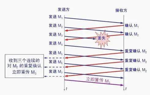
Assuming the receiver received M1 and M2 and sent acknowledgments for both. Now suppose the receiver did not receive M3 but then received M4.
Clearly, the receiver cannot acknowledge M4 because M4 is an out-of-order segment. According to the principles of reliable transmission, the receiver can either do nothing or send a timely acknowledgment for M2.
However, according to the fast retransmit algorithm, the receiver should promptly send a duplicate acknowledgment for M2, allowing the sender to know early that segment M3 has not reached the receiver. The sender then sends M5 and M6. The receiver receives these two segments and also sends another duplicate acknowledgment for M2. Thus, the sender receives four acknowledgments for M2, three of which are duplicates.
The fast retransmit algorithm also stipulates that as soon as the sender receives three duplicate acknowledgments, it should immediately retransmit the unacknowledged segment M3 without waiting for the retransmission timer for M3 to expire.
Since the sender retransmits unacknowledged segments early, adopting fast retransmit can increase overall network throughput by about 20%.
Fast Recovery
-
When the sender continuously receives three duplicate acknowledgments, execute the “multiplicative decrease” algorithm, halving the slow start threshold ssthresh. -
Unlike slow start, the sender does not set cwnd to 1 but instead sets cwnd to the value of ssthresh after halving and then begins executing the congestion avoidance algorithm (“additive increase”), allowing the congestion window to increase slowly in a linear manner.