Simulation Design Framework for Multi-Sensor Fusion in Autonomous Target Detection Tasks at Sea

With the proliferation of inexpensive autonomous unmanned systems, the pace of maritime operations is accelerating.

Unmanned surface systems can attack high-value targets at a low cost. For example, the Ukrainian Navy’s MAGURA V5 unmanned surface vessel, which costs significantly less than a missile frigate, has successfully sunk several Russian naval platforms.

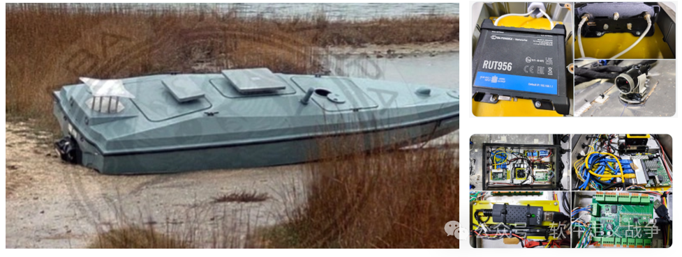
Magura-V5 Technical Specifications

Length: 5.5 meters (18 feet);

Width: 1.5 meters (5 feet);

Height above waterline: 500 mm (1.6 feet);

Cruising speed: 22 knots (41 km/h / 25.3 mph);

Maximum speed: 42 knots (78 / 48.3 mph);

Range: 450 nautical miles (833 km / 518 miles);

Payload: 320 kg (705.5 lbs);

Communication: Mesh wireless network with air relay or satellite communication.

Additionally, the Houthi forces have modified fishing boats into unmanned suicide boats, causing significant damage to commercial vessels and U.S. Navy escort ships.

These incidents highlight the threat posed by low-cost unmanned surface vessels to U.S. maritime power projection and economic assets.

Currently, there are no reliable defensive measures againstunmanned surface vessel threats, making the development of advanced target detection systems crucial.

Today, we introduce a study by the U.S. Navy. This study proposes an exploratory approach and simulation framework for modeling and evaluating multi-sensor suites against unmanned surface vessel threats.

The framework integrates sensors such as radar, LiDAR, optical, and thermal imaging sensors, combined with discrete-time state estimators for data fusion.

The simulation scenarios parameterize target kinematics, geometry, appearance, and environmental factors (sea conditions, lighting, precipitation, temperature) to generate noise measurements for each sensor at different sampling rates.

Target detection performance is quantified through normalization of position, speed, cross-sectional area, and color, aggregated into a composite index using user-defined weights.

The framework also employs Latin Hypercube Sampling (LHS) to explore sensor suite configurations and environmental conditions, identifying Pareto-optimal designs that balance accuracy and robustness.

This maritime unmanned autonomous target detection simulation framework’s materials can be downloaded by scanning the QR code below to join the circle. Document number in the circle:SDW152362 Simulation Design Framework for Multi-Sensor Fusion in Autonomous Target Detection Tasks at Sea

After joining the circle, search using the document number below, and you can also download other related materials in the circle:

《Task Engineering | Formal Construction and Quantitative Analysis Framework of Kill Chain》: SDW152361
《Situational Understanding and AI Explainability in Multi-Domain Warfare》: SDW152343
《Performance Optimization Pipeline for Tactical Edge AI Models》: SDW152342
《Generation of General Combat Maps Based on Multi-Agent Reinforcement Learning in Multi-Domain Warfare》: SDW152341
《Dynamic Code Adjustment of Unmanned Autonomous Systems in Complex Environments》: SDW152354
《AI Image Algorithms for Tactical Edge in Uncertain Battlefield Environments》: SDW152340
《Bayesian-Based Combat Testing》: SDW152336
《Hierarchical Reinforcement Learning-Based Digital Wargaming》: SDW152355
《Test Verification | Explainability Techniques for Verification Tools》: SDW152356

《Future Command Vision of the U.S. Army》: SDW152338
《AI Research Planning for Future Command of the U.S. Army》: SDW152339
《Explainability Analysis of Combat Mission Planning》: SDW152329
《Cognitive Models of Commanders and Measurement of Situational Awareness》: SDW152337
《Operational Test Verification of Situational Awareness》: SDW152333
《Building Command Information Flow in Unmanned Autonomous Systems of the U.S. Navy》: SDW152325

Related ReadingTask Engineering | Formal Construction and Quantitative Analysis Framework of Kill ChainShadow Command: Commander’s Digital Brain + Battlefield Simulation Software + Staff Intelligent AgentsTesting and Verification of AI Systems: Based on Digital Twins, Monte Carlo Simulation, and Synthetic DataJoint Test Concept Analysis under Joint All-Domain OperationsExplainability Research of Combat Mission Planning for Unmanned Autonomous SwarmsOrigins of Networks, Container Images, Microservices, Data, and Cybersecurity in Command SystemsBuilding Command Information Flow in UAV+UUV Distributed Unmanned Autonomous SystemsDigital Twin Systems Based on Reduced-Order Models, High-Fidelity Physics Models, and Uncertainty QuantificationTesting and Verification | “Virtual” Combat Testing Based on Modeling Simulation and Statistical Meta-ModelsTesting and Verification | Combat Testing Based on Bayesian MethodsOperational Test Verification of Situational Awareness under Joint All-Domain CommandAutomated Testing and Verification of Unmanned Autonomous Systems Based on SimulationOntology Design of Tasks and Capabilities of the SystemFuture Command of the U.S. Army (I): Vision and Impact of AI CommandFuture Command of the U.S. Army (III): In-Depth Understanding of AI-Based Command Systems1. Introduction

1.1 F2T2EA Kill Chain Against USV Threats

To effectively counter threats, the F2T2EA kill chain must remain intact. Any disruption at any stage will slow down response times.

The kill chain depicted in the figure was originally designed for anti-ship missiles, but its concept is equally applicable to USV threats. The yellow dashed line in the figure represents the target detection and tracking phase.

Improving the efficiency of the target detection phase can accelerate the entire kill chain, providing decision-makers with more time and intelligence to counterunmanned surface vessels.

1.2 Current Maritime Target Detection Capabilities

Current maritime detection relies on a layered sensor and platform architecture, with each platform having its unique advantages and inherent limitations.

Manned Surface Vessels: For example, the U.S. Coast Guard’s Sentinel-class Fast Response Cutter (FRC), while having a long endurance and some self-sustainability, requires regular returns for resupply and maintenance, reducing continuous coverage capability.

Unmanned Aerial Vehicles: Such as the AR5 EVO drone, capable of staying at sea for 16 hours, but limited by fuel or battery capacity, frequent shipboard launch/recovery cycles, and sensitivity to ice, strong winds, and precipitation.

Space Sensors: Such as optical and synthetic aperture radar (SAR) satellites, providing global coverage but with revisit intervals ranging from hours to days, and are easily affected by cloud cover, leading to intermittent target detection.

Over-the-Horizon Radar (OTHR): Capable of detecting surface targets over 1000 nautical miles, but with low spatial resolution, high infrastructure costs, and sensitivity to ionospheric variations and sea clutter.

Autonomous Fixed Sensor Platforms: Equipped with sensor payloads, autonomous fixed sensor platforms can provide continuous, unattended maritime monitoring. They can achieve near-real-time detection in localized areas, suitable for long-term surveillance in specific maritime regions. However, their coverage is limited, requiring multiple platforms for wide coverage, and they are sensitive to environmental conditions (such as sea state, precipitation).

Detection Platform Type	Main Features	Advantages	Limitations
Manned Surface Vessels	Such as the Coast Guard’s Sentinel-class Fast Response Cutter	Long endurance	Requires regular returns for resupply and maintenance
Unmanned Aerial Vehicles	For example, the AR5 EVO drone	Can stay at sea for extended periods (e.g., 16 hours)	Limited by fuel or battery capacity
Space Sensors	For example, optical and synthetic aperture radar (SAR) satellites	Provide global coverage	Revisit intervals of hours to days
Over-the-Horizon Radar (OTHR)	– Capable of detecting surface targets over 1000 nautical miles	Wide coverage	Low spatial resolution
Autonomous Fixed Sensor Platforms	Equipped with sensor payloads	Provide continuous, unattended maritime monitoring	Limited coverage

1.3 Research Objectives and Framework

To develop a method and tools for modeling and evaluating multi-sensor detection suites against USV threats. Through data fusion, overcome the failure issues of individual sensors in harsh sea conditions, low visibility, or complex environments.

This framework can simulate sensor behavior, environmental effects, and support sensor suite design using data fusion algorithms. It supports large-scale design space exploration by parameterizing simulation environments and sensor platforms.

2. Simulation Framework Description

This simulation framework proposes a systematic approach to evaluate sensor suites for unmanned surface vessel (USV) threat detection by simulating different sensor configurations and environmental conditions, thereby finding the optimal sensor suite that achieves the best balance between accuracy and robustness.

The main components of the framework include:

Environmental Simulator: Generates the real state of the USV and contextual information about the surrounding environment. This information drives sensor models and state estimators. The environmental simulator allows users to define the USV’s trajectory, color, geometry, and environmental parameters (such as lighting, precipitation, temperature, and sea conditions).
Sensor Models: Includes models for radar, LiDAR, optical cameras, and thermal imaging cameras, as well as a general sensor model.
Data Fusion Module: Implements algorithms such as Extended Kalman Filter (EKF) and Recursive Least Squares for fusing data from different sensors to estimate the USV’s position, speed, color, and cross-sectional area.
Performance Evaluation Module: Calculates the errors of the sensor suite across different performance metrics, normalizes them, and aggregates them into a composite performance index (P). This allows users to compare the performance of different sensor configurations.
Design Space Exploration Module: Uses Latin Hypercube Sampling (LHS) to explore the design space of sensor configurations and environmental conditions to identify Pareto-optimal designs that balance accuracy and robustness.
Result Visualization: Provides animations and charts to display the real position of the USV versus estimated position, color estimates, cross-sectional area estimates, and uncertainties in sensor measurements.

2.1 Environmental Simulator

The environmental simulator generates the actual state of the USV and contextual information about the surrounding environment, which drives sensor models and state estimators, determining the quality of measurements for each sensor suite.

The environmental simulator allows users to customize the USV’s trajectory, color, geometry, and environmental parameters (such as lighting, precipitation, temperature, and sea conditions).

Initialization Parameters: Users provide the following parameters at the start of the simulation:

Trajectory Parameters: Users define the USV’s trajectory by providing trajectory parameters A, B, C, D, E to define the position function of the USV on the x and y axes.

Color: Represented in the HSI color model by hue, saturation, and intensity.

Geometry: Assuming the USV is a rectangular prism with a height equal to the freeboard height.

Environmental Parameters: Including lighting, precipitation, temperature, and sea conditions, all of which are normalized continuous values relative to the baseline USV.

Simulation Case Class: This class is responsible for executing the following operations:

Enforce maximum values for trajectory coefficients (e.g., maximum speed and acceleration).
Calculate the initial polar coordinates of the USV based on user-defined heading and maximum range.
Inject environmental settings into each sensor instance.
Initialize data fusion state estimators for simultaneous estimation of kinematic and non-kinematic states.

2.2 Workflow of the Simulation Framework

Initialization: Users define the USV’s trajectory, color, geometry, and environmental parameters. The simulation framework initializes sensor models and data fusion algorithms based on these parameters.
Simulation Run: At each discrete time step, the simulation framework updates the real state of the USV, generates noisy measurements through sensor models, then uses data fusion algorithms to update state estimates and records real values and estimated values along with errors at each step.
Performance Evaluation: After the simulation ends, the framework calculates the normalized time average error for each performance metric and aggregates it into a composite performance index (P). Additionally, the framework generates probability density functions to show the performance distribution of different sensor suites across various scenarios.
Result Analysis: Users can evaluate and select the optimal sensor suite based on the composite performance index (P) and probability density functions. The framework also provides detailed diagnostic and debugging information to help users understand the simulation results.

2.3 Operations at Each Simulation Time Step

At each discrete time step, the simulation environment performs the following operations:

Real State Propagation: Updates the real state of the USV, including position, speed, and acceleration.
Real Cross-Sectional Area and Direction Calculation: Calculates the real cross-sectional area and direction of the USV.
Sensor Measurement Generation: Passes the real values through each sensor model to generate noisy measurements.
Data Fusion Algorithm Update: Uses data fusion algorithms (such as Extended Kalman Filter EKF) to update state estimates.
Data Recording: Records real values, estimated values, and errors at each step.
Global Time Step Alignment: Since different sensors may have different sampling rates, the simulation environment uses the greatest common divisor of all sensor intervals as the global time step to align the sampling of different sensors.

2.4 Simulation Termination and Output

The simulation terminates when the USV leaves the maximum range or reaches the simulation time limit.

After the simulation ends, the framework performs the following operations:

Output CSV File: Generates a time series CSV file containing all real and estimated states (position, speed, acceleration, cross-sectional area, direction, and color), measurements from each sensor, uncertainty radii, and errors at each step.
Performance Evaluation Metrics: Calculates and outputs an overall, subjectively weighted performance evaluation metric that aggregates error information into a composite measure for assessing the effectiveness of the scenario.
Diagnostic/Debugging Files: Generates diagnostic and debugging files that record initial parameters and termination conditions.
Animations and Plots (Optional): If the animation flag is enabled, the simulation will also generate the following animations and plots:

Polar Plot Animation: Displays the real versus estimated position of the USV (including USV heading arrows, real and estimated position indicators, one standard deviation uncertainty circles for the USV position, and floating sensor suite position markers).
Time Series Plot: Displays time series plots of position, speed, Kalman uncertainty, individual sensor uncertainty, and mean squared error (MSE).
Color Wheel Animation: Compares real and estimated HSI values.
Cross-Sectional Area Animation: Compares the real rectangular prism projection with the equivalent area circle’s cross-sectional area.

2.5 Batch Simulation

Batch Running: An automated script can read text file inputs of multiple parameter sets, generate corresponding instances of the simulation case class, and run them in batch mode for comparison across different sensor configurations and scenarios.
Parallel Processing: The framework has CUDA and CPU capabilities, allowing for parallel execution of each simulation case using a thread pool to improve simulation efficiency.

2.6 Features of the Simulation Framework

Flexibility: Users can customize sensor configurations, environmental conditions, and performance metric weights to suit different task requirements.
Comprehensiveness: Considers various sensor types and environmental factors, enabling a comprehensive assessment of sensor suite performance.
Data Fusion: Advanced data fusion techniques improve the accuracy of USV state estimation.
Design Space Exploration: Using Latin Hypercube Sampling (LHS) methods, efficiently explores the design space to find optimal sensor suite configurations.
Visualization: Provides rich visualization tools to help users intuitively understand simulation results.

Through this exploratory approach and simulation framework, researchers can systematically evaluate and select the most suitable sensor suite for specific task requirements to enhance detection and tracking capabilities for unmanned surface vessels (USVs).

3. Sensor Simulation Models

Sensor simulation models are the core components of the entire simulation framework, used to simulate the target detection performance of different sensors under various environmental conditions.

3.1 Classification of Sensor Models

Sensor Type	Main Function	Key Parameters
Radar	Detects target distance by emitting radio waves and receiving reflected waves	Transmit power, antenna gain, radar wavelength, target radar cross-section, distance, system noise temperature, receiver bandwidth, total loss factor
LiDAR	Generates 3D point clouds by emitting laser pulses and receiving reflected light	Transmit power, antenna gain, laser wavelength, target reflectivity, distance, detector quantum efficiency, pulse energy, incident angle, transmitter aperture diameter, receiver aperture area, beam divergence angle, noise figure, noise equivalent irradiance
Optical Camera	Generates images by capturing visible light reflected from targets	Target distance, target speed, ambient lighting, instantaneous field of view (IFOV), target angular size
Thermal Imaging Camera	Generates images by capturing thermal radiation emitted from targets	Target distance, target speed, ambient lighting, target thermal radiation intensity
General Sensor	Simulates user-defined sensor characteristics	User-defined sensitivity curves (sensitivity to sea conditions, precipitation, lighting, or temperature)

3.2 Factors Affecting Sensor Model Performance and Sources of Error

Sensor Type	Performance Influencing Factors	Sources of Error
Radar	Distance increases signal attenuation and noise increases	Reduced signal-to-noise ratio leads to increased measurement uncertainty
LiDAR	Distance increases, reflectivity decreases, beam divergence leads to signal attenuation	Reduced signal-to-noise ratio leads to increased measurement uncertainty, maximum effective range is limited
Optical Camera	Insufficient lighting, increased target distance, and high target speed lead to image blurriness	Insufficient or excessive ambient lighting, target distance being too far leads to increased errors
Thermal Imaging Camera	Ambient temperature can obscure thermal radiation, increased target distance leads to signal attenuation	Environmental temperature interference, target distance being too far leads to increased errors
General Sensor	User-defined noise factors and sensitivity curves	Measurement errors caused by user-defined noise curves

Each type of sensor corresponds to specific mathematical models, detailed in the original text.4. Data Fusion4.1 Data Fusion Metrics

Metric Name	Description	Importance
Position Estimation Error	Evaluates the accuracy of the sensor suite’s estimation of the USV’s position	High-precision position estimation is crucial for target tracking and decision-making
Speed Estimation Error	Evaluates the accuracy of the sensor suite’s estimation of the USV’s speed	Speed information helps predict the target’s future position and movement trends
Color Estimation Error	Evaluates the accuracy of the sensor suite’s estimation of the USV’s color (hue, saturation, intensity)	Color information can be used for target identification and classification
Cross-Sectional Area Estimation Error	Evaluates the accuracy of the sensor suite’s estimation of the USV’s cross-sectional area	Cross-sectional area information helps determine the target’s size and type
Composite Performance Metric P	Provides a composite evaluation value by weighted averaging the normalized errors of multiple performance metrics	The composite performance metric P reflects the overall performance of the sensor suite across multiple performance dimensions
Robustness	Evaluates the stability and reliability of the sensor suite under different environmental conditions	A robust sensor suite can maintain good performance in various complex environments

4.2 Data Fusion Methods

Data Type	Fusion Method	Main Objective	Key Features
Kinematic Data	Extended Kalman Filter (EKF)	Estimate the position and speed of the USV	Handles sensor data with different sampling rates, updates state estimates in real-time
Non-Kinematic Data	Recursive Least Squares	Estimate the color (H, S, I) and cross-sectional area of the USV	Assumes color values are relatively constant, updates estimates using Kalman gain

4.3 Error Handling in Data Fusion

4.3.1 Error Handling in Kinematic Data Fusion

Objective: Kinematic data fusion primarily focuses on estimating the position and speed of unmanned surface vessels (USVs).
Sources of Error:

Sensor Noise: Measurement data from each sensor (such as radar, LiDAR) contains noise, which affects the accuracy of position and speed estimates.
Environmental Factors: Environmental conditions such as sea state, precipitation, and temperature can affect sensor performance, further increasing measurement errors.
Model Inaccuracy: Kinematic models may not fully accurately describe the actual motion of the USV, leading to prediction errors.

Handling Methods:

Extended Kalman Filter (EKF): Through state update and measurement update steps, EKF can estimate the position and speed of the USV in real-time and use Kalman gain to weigh the reliability of sensor measurements and model predictions, thereby reducing errors.
Error Quantification: Quantifies the errors in position and speed estimates by calculating statistical measures such as root mean square error (RMSE) to assess and compare the performance of different sensor suites.
Environmental Adaptability: Considers the impact of environmental factors on sensor performance during data fusion, improving estimation robustness by adjusting parameters such as Kalman gain.

4.3.2 Error Handling in Non-Kinematic Data Fusion

Objective: Non-kinematic data fusion primarily focuses on estimating the color (hue, saturation, intensity) and cross-sectional area of the USV.
Sources of Error:

Sensor Noise: Measurement data from sensors such as optical and thermal imaging cameras also contains noise, which affects the accuracy of color and cross-sectional area estimates.
Environmental Factors: Environmental factors such as lighting conditions and temperature can affect sensor performance, further increasing measurement errors.
Model Inaccuracy: Non-kinematic models may not fully accurately describe changes in the USV’s color and cross-sectional area, leading to prediction errors.

Handling Methods:

Recursive Least Squares: Used to estimate the USV’s color values, assuming color values are relatively constant, recursively updating estimates to reduce errors.
Moving Average Method: For cross-sectional area estimation, uses a moving average method to average the most recent measurement values, reducing the noise impact of the current measurement.
Error Quantification: Quantifies the errors in color and cross-sectional area estimates by calculating statistical measures such as root mean square error (RMSE) to assess and compare the performance of different sensor suites.
Environmental Adaptability: Considers the impact of environmental factors on sensor performance during data fusion, improving estimation robustness by adjusting model parameters.

4.3 Detailed Steps for Data Fusion

Fusion Method	Steps	Description
Kinematic Data Fusion	State Update	Uses the system kinematic model to integrate the USV’s speed to predict position changes
Kalman Gain Calculation	Calculates Kalman gain based on sensor error characteristics (such as position, speed, precipitation, temperature, sea conditions, lighting)
Measurement Update	When the sensor provides new measurement data, calculates measurement residuals and updates state estimates
Non-Kinematic Data Fusion	Color Estimation	Uses recursive least squares to estimate the USV’s color values (H, S, I), assuming color values are relatively constant
Cross-Sectional Area Estimation	Uses a moving average method to average the most recent 20 measurement values, reducing the noise impact of the current measurement

5. Case Study Analysis

5.1 Case 1: Selecting the Best Performing Sensor Suite Under Specific Tasks

5.1.1 Background and Objectives

Background: Assume that enemy unmanned surface vessels (USVs) may attack the port of San Francisco under specific trajectories, at specific times, and under specific weather conditions. It is necessary to determine which sensor suite performs best under these specific conditions.

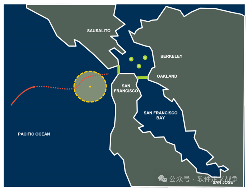
Objectives: Compare the performance of three predefined sensor suites under fixed task conditions to select the most suitable sensor configuration for the task.

5.1.2 Sensor Suite Configurations

Sensor Suite	Configuration Description
Low-Quality Radar	Contains only one low-quality radar
High-Quality Radar	Contains only one high-quality radar
Mixed Suite	Contains one medium-quality radar, LiDAR, optical camera, and thermal imaging camera

5.1.3 Simulation Scenario Settings

USV Trajectory: The USV starts from a distance, crosses the detection range of the sensor suite (marked as a buoy), and moves to the right. The trajectory is defined by specific coefficients, allowing for the simulation of different motion patterns in the simulation.
Environmental Conditions: Specific time, weather, and sea conditions that remain constant in the simulation to ensure fairness in comparison.

5.1.4 Simulation Results

Position Estimation:

Low-Quality Radar: Position estimation error is large.
High-Quality Radar: Performs well at close range but not as well as the mixed suite at long range.
Mixed Suite: Performs best across all position estimates, with the smallest error.

Speed Estimation:

Low-Quality Radar: Speed estimation error is large.
High-Quality Radar: Speed estimation error is similar to the mixed suite, but performs better in some cases.
Mixed Suite: Speed estimation error is small and performance is stable.

Color Estimation:

Low-Quality Radar: Cannot measure color, so there is no color estimation error data.
High-Quality Radar: Also cannot measure color, so there is no color estimation error data.
Mixed Suite: Able to measure color, with the smallest color estimation error, performing best.

Cross-Sectional Area Estimation:

Low-Quality Radar: Cross-sectional area estimation error is large.
High-Quality Radar: Cross-sectional area estimation error is small, performing well.
Mixed Suite: Cross-sectional area estimation error is between the two, performing well.

5.1.5 Composite Performance Evaluation

Performance Metric P: Uses normalized time average error to quantify the performance of the sensor suite and aggregates these errors into a composite performance metric P based on user-defined weights.
Evaluation Results:

Mixed Suite: Composite performance metric P is 0.750078, performing best, especially with a significant advantage in color measurement.
High-Quality Radar: Composite performance metric P is 2.88357, performing well, but cannot compete with the mixed suite in color measurement.
Low-Quality Radar: Composite performance metric P is 3.48851, performing the worst.

5.1.6 Conclusion of Case 1

Mixed Suite performs best under specific task conditions, especially with a significant advantage in color measurement. High-quality radar performs well in position and speed estimation but cannot measure color, which may be a critical performance metric in some tasks.
Low-Quality Radar performs the worst across all performance metrics, indicating that quality is an important consideration when selecting sensor suites.
Composite Performance Metric P provides a comprehensive evaluation method, allowing users to weight different performance metrics based on specific task requirements to select the most suitable sensor suite.

5.2 Case 2: Design Space Exploration of Sensor Suites Under Various Environmental Conditions

5.2.1 Background and Objectives

Background: In practical applications, it is necessary to design a sensor suite that can operate robustly under various environmental conditions, not just one that performs best under specific conditions. Therefore, it is necessary to explore different sensor configurations to find sensor suites that can provide reliable performance across multiple scenarios.

Objectives: To explore the design space of sensor configurations and environmental conditions using the Latin Hypercube Sampling (LHS) feature of the simulation framework to identify sensor suites that achieve the best balance between accuracy and robustness.

5.2.2 Sensor Suite Configurations

Users defined three sensor suite configurations, each containing different numbers and qualities of sensors. The specific configurations are as follows:

Sensor Suite	Configuration Description
Sensor Suite 000	1 medium-quality radar, 1 medium-quality LiDAR, 2 medium-quality optical cameras, 1 medium-quality thermal imaging camera
Sensor Suite 001	1 low-quality radar, 2 low-quality LiDARs, 1 high-quality optical camera, 2 low-quality thermal imaging cameras
Sensor Suite 002	2 low-quality radars, 2 high-quality LiDARs, 1 low-quality optical camera, 2 high-quality thermal imaging cameras

5.2.3 Simulation Scenario Settings

Environmental Conditions: Randomly varying sea states, lighting, precipitation, and temperature to test the robustness of the sensor suites under different environmental conditions.
USV Trajectory: Fixed trajectory, but environmental conditions vary randomly.
Number of Test Scenarios: Each sensor suite runs 1000 scenarios to test its robustness.

5.2.4 Simulation Results

Performance Evaluation: Uses normalized time average error to quantify the performance of the sensor suites and aggregates these errors into a composite performance metric P based on user-defined weights.
Probability Density Functions: Generates probability density functions for each sensor suite to show their performance distribution across various scenarios.
Results:

Sensor Suite	Average Error	Standard Deviation	Composite Performance Metric P
Sensor Suite 000	0.6245	0.3103	Best Performance
Sensor Suite 001	0.6492	0.3383	Worst Performance
Sensor Suite 002	0.6339	0.3161	Good Performance

5.2.5 Result Analysis

Sensor Suite 000: Performs most robustly across various scenarios, with the lowest average error and standard deviation. This indicates that a combination of medium-quality sensors can provide good robustness.
Sensor Suite 001: Contains multiple low-quality sensors and performs the worst. This indicates that a combination of low-quality sensors may not provide sufficient robustness across various scenarios.
Sensor Suite 002: Although it contains multiple high-quality sensors, its performance is similar to 000. This indicates that a combination of high-quality sensors can provide good performance in some cases but may require more resources.

5.2.6 Conclusion of Case 2

Balance of Robustness and Accuracy: Through design space exploration, users can identify sensor suites that perform optimally under various scenario conditions. Case 2 indicates that a combination of medium-quality sensors (such as Sensor Suite 000) achieves a good balance between robustness and accuracy.
Importance of Redundancy: Redundant sensor configurations can enhance system robustness, especially when facing various environmental conditions. The performance of Sensor Suites 000 and 002 indicates that redundant high-quality sensors can significantly improve overall system performance.
Composite Performance Metric P: Provides a comprehensive evaluation method, allowing users to weight different performance metrics based on specific task requirements to select the most suitable sensor suite.

6. Conclusion

6.1 Research Findings

Performance Evaluation: Through two case studies, the capabilities of the simulation framework are demonstrated. Case 1 compared the performance of predefined sensor suites under specific task conditions, while Case 2 explored the design space to identify sensor suites that perform optimally under various scenario conditions.

Key Findings:

Mixed Sensor Suites perform best under specific task conditions, especially with a significant advantage in color measurement.

Medium-Quality Sensor Combinations provide good robustness and accuracy across various scenarios.

Redundant Sensor Configurations can significantly improve overall system performance, especially when facing various environmental conditions.

6.2 Significance of the Research

A systematic approach is proposed for designing and evaluating sensor suites against USV threats, providing a powerful tool for countering autonomous system threats.

Through design space exploration, sensor suites that perform optimally under various scenario conditions are identified, providing a scientific basis for sensor selection in practical applications.

6.3 Future Work

Sensor Model Calibration: Calibrate sensor models through experimental and testing platforms to improve model accuracy and reliability.
Enhanced Sensor Physics and Modeling: Introduce higher fidelity sensor models, including proprietary sensor characteristics and additional sensor types.
Cost and Power Consumption Analysis: Incorporate cost and power consumption as additional design weights in design space exploration to support more comprehensive sensor suite evaluations.
Expanding Application Areas: Extend the framework to underwater, ground, and aerial applications to address a broader range of autonomous system threats.