💡 Introduction to Optimization: Tackling Unconstrained One-Dimensional Extremum Problems!

Hello everyone! Welcome to our optimization knowledge classroom! 🚀

In the vast realm of numerical computation and engineering design, “optimization” is a ubiquitous core topic. Whether it’s about making rockets fly higher, algorithms run faster, or maximizing investment returns, there often lies an optimization problem. Today, we will start with the most fundamental and important type of problem—unconstrained one-dimensional extremum problems, and together we will unveil its mysterious veil!

🎯 Problem Background: What Are We Trying to Solve?

The “unconstrained one-dimensional extremum problem” we are going to discuss can be simply described in mathematical terms as solving problems of the following form:

Here, is a one-dimensional variable (think of it as a point on the number line), and is a function associated with this variable (for example, or). Our goal is to find the value of that allows the function to achieve its minimum value (or “local minimum”).

Please note, the term “unconstrained” here means that the variable is not subject to additional constraints (for example, must be greater than 0, etc.).

There are two main cases:

1. 1. Global Optimization: If the range of the independent variable is the entire real line, then we are looking for the global minimum of the function. This case is usually more complex, and we will not delve into it in this book for now.
2. 2. Local Optimization or Interval Optimization: In this chapter, we focus on the following two more common and fundamental situations:

• • Given that the range of the independent variable is the entire real interval, find any local minimum point of the function .
• • Given that the range of the independent variable is limited to a specified closed interval, find any local minimum point of the function within this interval.

So, how do we start solving such problems? A commonly used tool is the one-dimensional search method.

One-dimensional search, as the name suggests, is to search for the extremum point of the target function along a certain known direction (in one-dimensional problems, this direction is either the positive or negative direction of the number line). Its core idea is iteration: based on the information from the currently known point, calculate a new, better point (i.e., a point with a smaller function value) step by step, approaching the extremum point we want to find.

There are various methods for one-dimensional search, which can be quite diverse! Depending on the order of information that the iterative formula relies on, they can be roughly divided into two main categories:

• • Line Search: This type of method mainly utilizes function values or first-order derivative information. Common representatives include:
• • Golden Section Method
• • Fibonacci Method
• • Newton’s Method
• • Non-linear Search: This type of method may use higher-order information or perform function approximation. Common representatives include:
• • Parabolic Interpolation
• • Cubic Interpolation

However, before formally applying these sophisticated search methods, we often need to do one very important thing—determine a search interval that roughly contains the extremum point. Just like treasure hunting, you need to know roughly where the treasure is located, right?

Next, we will first introduce a classic algorithm specifically used to determine this initial search interval—the Advance-and-Retreat Method. This method, although simple, is very crucial! Because it can provide a reliable starting point for our subsequent fine searches (such as the Golden Section Method, Newton’s Method, etc.), ensuring that we do not “go in the wrong direction” or “miss the target.” The Advance-and-Retreat Method itself is also an indispensable part of various more complex optimization methods when searching for the direction of iterative descent.

Are you ready? Let’s dive into how the “Advance-and-Retreat Method” helps us “pinpoint” the hiding place of the extremum point! 🔍

6.1 The Advance-and-Retreat Method: The Magic Tool for Locking Down the Extremum’s Hiding Interval 🔍

1. Algorithm Principle: Between Advance and Retreat, the Interval Emerges

The Advance-and-Retreat Method aims to find an initial search interval that contains the target function’s extremum point. The theoretical basis behind it is quite intuitive, mainly relying on the properties of unimodal functions.

What is a unimodal function? Simply put, it is a function that has only one extremum point within a certain interval, shaped like a valley with only one lowest point (the “bottom of the valley”).

For such a unimodal function , if we already have a search interval that contains its extremum point, then:

For any two points taken within the interval :

• • If , this means that is lower than , then the extremum point (the bottom of the valley) cannot possibly be to the right of and must be located within the interval .
• • If , this means that is lower than , then the extremum point cannot possibly be to the left of and must be located within the interval .

Utilizing this property, the Advance-and-Retreat Method can start from an initial point and an initial step size , and through exploratory “advancing” and “retreating,” gradually determine the search interval. The specific process is as follows:

1. 1. Advance one step: First, calculate the function values at the initial point and one step forward , i.e., and . Then compare their sizes:
2. 2. Determine the direction and adjust the interval:

• • Case 1: If indicates that we have “climbed higher” by taking a step forward, then the extremum point (the bottom of the valley) is likely “behind us” or right here. At this point, we know that the right endpoint of the search interval can be set to , but the left endpoint is still uncertain. What to do? We need to retreat! Starting from , calculate by multiplying the step size by a certain reduction factor (usually , for example, taking ). If is still less than or equal to , it indicates that we have not yet found the “uphill” trend and may need to continue retreating (or adjust the ). Until we find a suitable such that , this indicates that we have moved from the “bottom of the valley” to another direction “uphill.” Thus, we have successfully determined the search interval containing the extremum point:.
• • Case 2: If (Note: The original text is >, but including = is more rigorous; actual algorithm implementations usually imply >=), this indicates that we have “descended” by taking a step forward, or reached a lower place! This suggests that the extremum point (the bottom of the valley) is likely still ahead. At this point, we know that the left endpoint of the search interval can be set to , but the right endpoint still needs exploration. What to do? We need to continue to advance! However, to find the other end of the interval more quickly, we usually increase the step size. For example, by multiplying the enlargement factor (usually , for example, taking ) by the current step size (note that the step size may change during iterations, and the subsequent algorithm steps will elaborate), calculate . If is still less than or equal to , it indicates that we are still continuing “downhill” or are in a flat area, and we need to continue advancing (possibly also continue to enlarge the step size). Until we find a suitable (and a possibly enlarged step size), such that (or more accurately, comparing two consecutive steps), this indicates that we have crossed the “bottom of the valley” and started “uphill.” Thus, we have determined the search interval:. (The specific method for determining the interval endpoints can be found in the algorithm steps.)

Through this advance and retreat (or continuous forward/backward) exploration, we can ultimately lock down an effective interval containing the extremum point.

2. Principle Explanation: Deep Understanding, Clarity!

To help everyone better understand the essence of the Advance-and-Retreat Method, let’s analyze it from several angles:

1. Visual Understanding (Valley Metaphor) ⛰️

• • Imagine you are in a continuous valley, and your task is to find the lowest point (extremum point) of the valley.
• • Your function is like the elevation at different positions in the valley. We assume this valley is relatively regular and is unimodal, meaning it has only one unique lowest point.
• • You start from an initial position, holding a initial step size measuring rod.
• • You take a step forward or backward (the step size is a multiple of or ) and measure the elevation at your current position.
• • The key lies in comparison: By comparing the elevations of your two steps, you can determine whether the lowest point is roughly in the direction you are advancing or retreating, thus narrowing down the range in which you are searching for the lowest point.

2. Mathematical Principle (Core Inequality) 📈

The mathematical foundation for the effectiveness of the Advance-and-Retreat Method is the key property of unimodal functions:

For unimodal functions , within an interval that contains the extremum point, for any two points taken :

• • ✅ If , then the extremum point must fall within the interval (because to the right will only be higher).
• • ✅ If , then the extremum point must fall within the interval (because to the left will only be higher).

It is this simple comparison rule that guides every decision made by the Advance-and-Retreat Method.

3. Detailed Algorithm Steps (Breaking Down Two Cases) ⚙️

Let’s take a closer look at the logical behavior of the algorithm in the two main cases:

Case 1: (Initial Backward Search Trend)

   <--- Searching for the left boundary --- x₀ --- Testing forward ---> x₀+h
          ?             | (lower point)         | (higher point)
                        f(x₀)    <      f(x₀+h)

1. 1. Calculate: First calculate and .
2. 2. Compare: Find that . This suggests that the extremum point may be to the left, or itself is the extremum point.
3. 3. Retreat Exploration: Starting from , test in the negative direction (left side) with a step size of (or ) to explore. Calculate (or ).
4. 4. Find the Turning Point: Continue retreating until finding a point such that . (Note: In actual algorithm implementations, it is usually necessary to compare two consecutive steps, such as to determine whether to start “uphill”).
5. 5. Determine the Interval: Once this “uphill” sign is found, it indicates that we have crossed the extremum point area. The final determined interval containing the extremum point is usually (or determined by the algorithm steps).

Case 2: (Initial Forward Search Trend)

   x₀ --- Testing forward ---> x₀+h --- Continue forward ---> x₀+λh ...
   | (higher point)         | (lower point)          ?
   f(x₀)    >=     f(x₀+h)

1. 1. Calculate: Calculate and .
2. 2. Compare: Find that . This strongly suggests that the extremum point is to the right, or itself is the extremum point.
3. 3. Forward Exploration: Starting from , continue testing in the positive direction (right side) with a step size of (usually also enlarging the step size, for example, or ) to explore. Calculate (or subsequent points).
4. 4. Find the Turning Point: Continue advancing and possibly enlarging the step size until finding a point such that . This marks that we have crossed the bottom and started “uphill”.
5. 5. Determine the Interval: At this point, the search interval containing the extremum point is usually (or determined by the algorithm steps).

4. Example Demonstration (Manually Simulating Once) ✍️

Assuming our target function is (this is an upward-opening parabola with its vertex at , which is clearly a unimodal function). We take the initial point , and the initial step size to simulate the Advance-and-Retreat Method:

1. 1. Calculate Initial Two Points:

• •
• •

2. Compare: . This belongs to Case 2, indicating that the extremum point is to the right, and we need to continue advancing.

3. Enlarge Step Size and Advance: We will enlarge the step size by times (i.e., the new step size is ). Starting from the current lower point , we move forward by the new step size , reaching .

• • Calculate .
• • Compare: and . Since is not greater than , we have not yet found the “uphill” point and need to continue advancing.

4. Again Enlarge Step Size and Advance: The step size is doubled again, becoming . Starting from the current point , we move forward by , reaching .

• • Calculate .
• • Compare:. Finally! We found a point that is higher than the previous step, indicating that we have crossed the bottom.

5. Determine the Interval: Based on the specific recording method of the algorithm (see the next section), the interval we found will include (the point before the descent) and (the point after the ascent), as well as the point in between . The final determined search interval may be or a similar range (the specific endpoints depend on the details of the algorithm steps, such as using which may be or or ). The important thing is that this interval [1, 7] indeed contains the true extremum point!

5. Precautions (Usage Tips) ⚠️

• • Choice of Initial Step Size: It should not be too large (which may directly skip the extremum point area) nor too small (which may slow down the search). It needs to be chosen based on the characteristics of the problem and experience.
• • Reduction/Enlargement Factor: Usually, the reduction factor is taken as or (related to the golden ratio), and the enlargement factor is taken as .
• • Function Requirements: Theoretically, the Advance-and-Retreat Method requires the function to be unimodal. If the function has multiple extremum points (multimodal), the Advance-and-Retreat Method can only guarantee finding an interval that contains some extremum point, not necessarily the global minimum.

3. Algorithm Steps: Programmatic Execution Flow

Below are the basic algorithm steps for using the Advance-and-Retreat Method to solve the one-dimensional unconstrained problem to find the search interval (the warm-hearted little interval that must contain some extremum point):

Initialization:

1. 1. Given an initial point , and an initial step size (must be a positive number).
2. 2. Set the current point .
3. 3. Set the current step size .
4. 4. Initialize the iteration count (or state marker) .

Iterative Search:

➡️ Step 2: Calculate the test point . And increase the iteration counter by 1 ().

➡️ Step 3: Calculate and . Compare their sizes:* If (the function value has decreased! Good sign!), it indicates that we may still be going downhill or just crossed the bottom, and need to continue advancing.Jump to Step 4.* Otherwise (i.e., ) (the function value has not decreased, but rather increased or remained the same), it indicates that we may have found the uphill trend, or we may have gone in the wrong direction from the start. We need to judge based on the situation.Jump to Step 5 to determine.

➡️ Step 4: (because )* Update Point: Save the original as (), and set the new lower point as the current ().* Update function value (optional, for efficiency): (old value), (new value).*Enlarge Step Size: Double the step size (), to accelerate forward.*Return to Step 2, using the new and enlarged step size to continue testing.

➡️ Step 5: (because and )* Check the value of :*If (this means that this is the first iteration that has found ), it indicates that the initial forward direction (step size ) may be wrong, and the extremum point is likely in the opposite direction of .Jump to Step 6 for reverse search.*Otherwise (i.e., ), it indicates that we have at least successfully advanced once (executed Step 4), and now we have finally encountered a situation where the function value has increased or remained the same. This indicates that we have found the “other end” of the interval containing the extremum point!Jump to Step 7 to end the search.

➡️ Step 6: (because and )*Reverse Step Size: Change the step size to a negative value ().* Record Point: Save the recently “failed” test point as (), while also saving its function value. (At this point, is still ).*Return to Step 2, using the current (i.e., ) and the reverse step size to restart testing.

➡️ Step 7: (because and )*Determine the Interval Endpoints: At this point, we should have three key points:(the last point that successfully descended or remained the same), (the previous point of , which is closer to the initial point or in the reverse direction), and (the point that caused the function value to first rise or remain the same).* Organize it, letting , , . (This is just to correspond with the final output form of some textbooks [x1, x3] or [x3, x1]; the variable reassignment here may differ slightly from the code implementation, but the key is to understand that we have found three boundary points of the interval).*Stop Calculation. We have successfully found an interval containing the extremum point! This interval is formed by the point that just caused the function value to rise and the point before it. The final search interval is defined by the coordinates of the points and , which may be or (depending on which value is smaller).

Through this “advance and retreat” maneuver, we have obtained a valuable interval that we can confidently hand over to subsequent more refined search algorithms!

4. Algorithm Implementation: Python Code Showcase Time! 🐍

The theory and steps have been clarified, and it is time to showcase the power of code! Below is the implementation of the Advance-and-Retreat Method function <span>minJT</span>, which accepts the target function <span>f</span>, the initial point <span>x0</span>, and the initial step size <span>h0</span> as inputs, and can optionally visualize the search process.

# <PYTHON>
import numpy as np
import matplotlib.pyplot as plt

def minJT(f, x0, h0, eps=1e-6, visualize=False):
    """
    Use the Advance-and-Retreat Method to solve the extremum interval of a one-dimensional function
  
    Parameters:
        f: Target function, callable object, accepts a numerical parameter
        x0: Initial point
        h0: Initial step size
        eps: Precision (optional, default 1e-6)  # Note: This eps parameter is usually not used in the Advance-and-Retreat Method, kept for interface uniformity or other purposes
        visualize: Whether to visualize results (optional, default False)
      
    Returns:
        (minx, maxx): Left and right endpoints of the interval containing the extremum (minx <= maxx)
    """

    # Record the search process for visualization
    search_points = [x0] if visualize else None
    search_values = [f(x0)] if visualize else None

    x1 = x0  # Initialize current point x^(1)
    k = 0     # Iteration counter
    h = h0    # Current step size

    # First, perform a test (corresponding to part of Step 2)
    x4 = x1 + h
    f4 = f(x4)
    f1 = f(x1) # Function value at the initial point

    if visualize:
        search_points.append(x4)
        search_values.append(f4)

    # Determine the initial search direction (corresponding to parts of Steps 3 and 5)
    if f4 >= f1: # Case 1: Encountered an increase or flatness at the initial step, need to reverse (corresponding to Step 6)
        h = -h   # Reverse step size
        x4 = x1 + h # Recalculate the test point in reverse
        f4 = f(x4)
        if visualize:
             search_points[-1] = x4 # Update the last test point to the reverse point
             search_values[-1] = f4
      
        # If the first reverse step still increases or remains the same, it indicates that the initial point may be near the extremum or the step size is too large. Directly return a small interval around the initial point
        if f4 >= f1: 
            print("Warning: Initial point might be near the minimum or step size is too large. Returning interval around x0.")
            minx = min(x0 - h0, x0 + h0) # Based on the original step size, give a small interval
            maxx = max(x0 - h0, x0 + h0)
            if visualize:
                _plot_search_process(f, minx, maxx, search_points, search_values)
            return minx, maxx
        # Otherwise, the reverse test is successful, enter the main loop to continue reverse search
        x2 = x1 # Save x0
        x1 = x4 # Update x1
        f2 = f1
        f1 = f4
        h *= 2# Double the reverse step size
        k = 1# Mark that we have reversed
    else: # Case 2: The initial step successfully descended, continue forward (corresponding to part of Step 4)
        x2 = x1 # Save x0
        x1 = x4 # Update x1
        f2 = f1
        f1 = f4
        h *= 2# Double the forward step size
        k = 1# Normal iteration

    # Main loop (continue executing Steps 2, 3, 4 until finding the uphill point)
    while True:
        x4 = x1 + h  # Test one step forward (or in reverse) (Step 2)
        f4 = f(x4)  # Calculate the function value at the test point
      
        if visualize:
            search_points.append(x4)
            search_values.append(f4)
      
        # Compare function values (Step 3)
        if f4 < f1:
            # Case 1: The function value at the test point is smaller, continue forward/reverse (Step 4)
            x2 = x1  # Save the previous point
            x1 = x4  # Update the current point
            # f2 = f1 # f2 seems unnecessary to update in real-time in this implementation; x3 will use it later
            f1 = f4
            h *= 2   # Increase step size
            k += 1
        else:
            # Case 2: Encountered an increase or flatness, found the interval (Step 7)
            break # Exit the loop
          
    # Determine the final interval endpoints (Step 7's organization part)
    # At this point, x1 is the last failed point, x2 is the previous successful descending point, and the previous point of x2 (i.e., the role of x3) is played by the last successful x2
    # The interval is defined by the point that caused the rise (x1) and the previous point (x2)
    minx = min(x1, x2) 
    maxx = max(x1, x2) 

    # The implementation here may not completely align with the description of x1, x3, but the final effect is to find an interval containing the extremum
    # If strictly following the description, assigning x1=x4, x3=x2 (the last successful x2), then the interval is [min(x4, last successful x2), max(x4, last successful x2)]
    # The current code's min(x1, x2) is equivalent to min(x4, last successful x4')
    # In fact, it is the interval formed by the last failed point and the second-to-last successful point, which is also valid

    if visualize:
        _plot_search_process(f, minx, maxx, search_points, search_values)

    return minx, maxx

def _plot_search_process(f, minx, maxx, points, values):
    """(Internal function) Visualize the search process"""
    plt.figure(figsize=(10, 6))

    # Generate function curve data points, the range should be large enough
    plot_range_min = min(min(points), minx) - abs(maxx-minx)*0.5 - 1
    plot_range_max = max(max(points), maxx) + abs(maxx-minx)*0.5 + 1
    x = np.linspace(plot_range_min, plot_range_max, 400)
    y = [f(xi) for xi in x] # Use list comprehension to support non-numpy native functions

    # Plot the function curve
    plt.plot(x, y, 'b-', label='Function Curve: $f(x)$')

    # Mark all points in the search process
    plt.scatter(points, values, c='r', s=50, zorder=5, label='Search Points ($x^{(k)}$)')

    # Use dashed lines to connect search points, showing the trajectory
    if len(points) > 1:
        plt.plot(points, values, 'r--', alpha=0.6, label='Search Path')
        # Mark the starting point
        plt.scatter(points[0], values[0], c='orange', s=100, edgecolors='black', zorder=6, label='Start Point ($x_0$)')

    # Mark the final found search interval
    plt.axvline(x=minx, color='g', linestyle='-.', linewidth=2, label=f'Interval Min ({minx:.2f})')
    plt.axvline(x=maxx, color='g', linestyle='-.', linewidth=2, label=f'Interval Max ({maxx:.2f})')

    # Mark the midpoint of the interval
    midpoint = (minx + maxx)/2
    plt.axvline(x=midpoint, color='purple', linestyle=':', linewidth=2, label=f'Midpoint ({midpoint:.2f})')

    # Add chart annotations and information
    plt.title('Interval Search using Advance-and-Retreat Method Visualization', fontsize=14)
    plt.xlabel('$x$', fontsize=12)
    plt.ylabel('$f(x)$', fontsize=12)
    plt.legend(fontsize=10)
    plt.grid(True, linestyle='--', alpha=0.7)
    plt.ylim(min(values)-abs(max(values)-min(values))*0.2, max(values)+abs(max(values)-min(values))*0.2) # Adjust y-axis range

    # Display key information text on the chart
    text_info = f'Initial point $x_0$: {points[0]:.3f}\n' 
                f'Initial step $h_0$: {abs(points[1]-points[0]) if len(points) > 1 else h0:.3f}\n' 
                f'Found interval: [{minx:.4f}, {maxx:.4f}]\n' 
                f'Interval length: {maxx-minx:.4f}\n' 
                f'Midpoint: {midpoint:.4f}'
    plt.text(0.03, 0.97, text_info, transform=plt.gca().transAxes, fontsize=10,
             verticalalignment='top', bbox=dict(boxstyle='round,pad=0.4', fc='wheat', alpha=0.5))

    plt.tight_layout() # Automatically adjust layout to prevent label overlap
    plt.show()

# --- Test Example ---
if __name__ == "__main__":
    # Define a test function f(x) = (x-2)^2 + 1, whose extremum point is at x=2
    def test_func(x):
        return (x - 2)**2 + 1

    # Set initial conditions
    x0 = 0    # Initial point
    h0 = 0.1 # Initial step size

    print(f"Starting Advance-and-Retreat search for f(x)=(x-2)^2+1 with x0={x0}, h0={h0}")

    # Call the Advance-and-Retreat Method function and enable visualization
    minx, maxx = minJT(test_func, x0, h0, visualize=True)

# Print results
    print(f"\nSearch complete.")
    print(f"Found interval: [{minx:.4f}, {maxx:.4f}]\n")
    print(f"Midpoint: {(minx + maxx)/2:.4f}")

This code not only implements the logic of the Advance-and-Retreat Method but also thoughtfully includes visualization functionality (<span>_plot_search_process</span> function), allowing us to intuitively see how the algorithm “advances and retreats” step by step to ultimately define the interval. Running this example, you will see a graph similar to the one below (the specific positions of the points and the interval will vary slightly based on the initial values):

5. Explanation: What Do the Results “Found Interval” and “Midpoint” Mean? 🤔

When you run the above Python code (or any other implementation of the Advance-and-Retreat Method), you will typically receive two key output messages: “Found Interval” and “Midpoint.” What do they represent? Let’s break it down for you:

📊 Found Interval [minx, maxx] (The Found Interval)

Explanation:<span>Found interval: [minx, maxx]</span> This output is the interval that the Advance-and-Retreat Method has locked down through a series of tests, which contains (at least one) extremum of the function.<span>minx</span> is the left endpoint of the interval, and <span>maxx</span> is the right endpoint of the interval.

Its importance is crucial:

• • ✅ Locking the Target: It tells you that the value that minimizes the function must be located between <span>minx</span> and <span>maxx</span>! It won’t run away!
• • 🎯 Subsequent Navigation: This interval acts like a “treasure map marking area,” serving as the initial base camp for subsequent more precise optimization algorithms (such as the Golden Section Method, Fibonacci Method, or Newton’s Method that we will discuss later). With this reliable starting point, subsequent fine searches can be more directed, greatly improving the efficiency and success rate of finding the precise extremum point, avoiding blind searches on the infinite number line.

For example: If the program outputs <span>Found interval: [0.8000, 3.2000]</span>, great! This means the extremum point is indeed contained within this interval, and the Advance-and-Retreat Method has successfully completed its task.

• • But if (due to improper initial point or step size settings) the output is <span>Found interval: [3.5000, 6.0000]</span>, then that’s bad; this interval does not contain the true extremum point. This reminds us to check the initial settings or whether the function itself meets the unimodal property.

📍 Midpoint (The Midpoint of the Interval)

Explanation:<span>Midpoint</span> is easier to understand; it is simply the midpoint of the interval <span>[minx, maxx]</span>, calculated using the formula <span>(minx + maxx) / 2</span>.

Its role is mainly auxiliary:

• • 💡 Initial Guess: The midpoint can be seen as a simple, preliminary estimate of the location of the extremum point. Although it is not necessarily the precise extremum point, it is often not too far away (especially when the interval is small).
• • 🚀 Accelerating Convergence: In subsequent more precise iterative searches (such as the Golden Section Method), this midpoint of the interval can sometimes be chosen as the initial point for iteration, which may converge to the final solution faster than starting from one of the endpoints of the interval.

For example:

• • If the found interval is <span>Found interval: [1.0000, 3.0000]</span>, then <span>Midpoint = (1.0 + 3.0) / 2 = 2.0</span>. Wow! This time the midpoint happens to be the extremum point we know! (Of course, this is usually a more ideal or coincidental situation).
• • If the found interval is <span>Found interval: [1.2000, 3.8000]</span>, then <span>Midpoint = (1.2 + 3.8) / 2 = 2.5</span>. This midpoint, while not the precise extremum point, also provides a starting point that is not far from the true solution.

🤔 Why Do We Need These Two Values?

To summarize, the value of the outputs from the Advance-and-Retreat Method lies in:

1. 1. <span>Found Interval</span>‘s Core Value:

• • Locking the Range, Ensuring No Solution is Lost: This is the primary task of the Advance-and-Retreat Method! Ensuring that the target extremum point is “netted” within this interval.
• • Avoiding Failure Risks: Providing an effective input for subsequent optimization algorithms (like the Golden Section Method) that rely on the interval, preventing them from failing due to incorrect initial intervals (where the target is not contained).

2. <span>Midpoint</span>‘s Auxiliary Value:

• • Providing a Starting Point: Giving the subsequent iterations a “not bad” initial guess position.
• • Roughly Assessing the Interval: In some complex cases, comparing the function values at the midpoint and endpoints may also provide clues about the approximate location of the extremum point within the interval.

📈 Analyzing with Visual Images (Using the Previous <span>test_func</span> as an Example)

Assuming you ran the code for <span>test_func</span>, you would get output and images similar to the ones below:

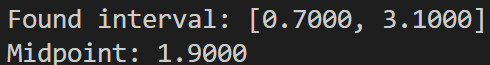
Output Results:

Visual Image:

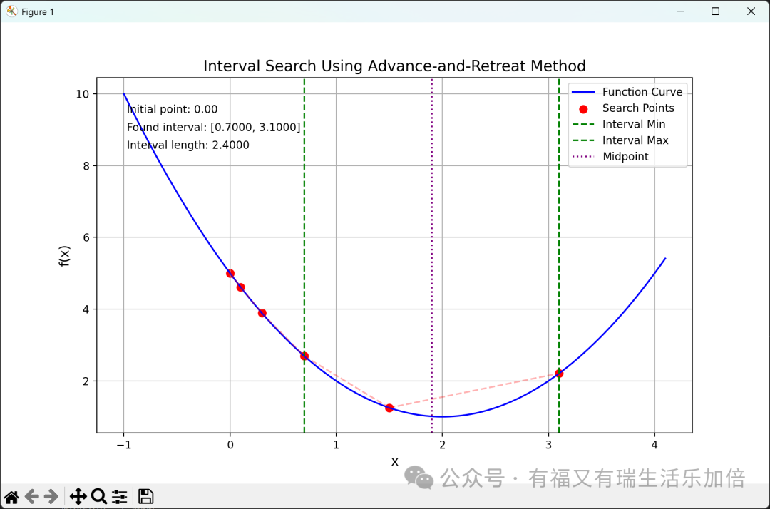
Interpreting This Image and Results:

1. 1. Red Points (Search Points) and Red Dashed Line (Search Path): Clearly show how the algorithm starts from the initial point <span>x0=0</span>, how it tests step by step (first to the right), and how the function value changes (first decreases and then increases) until it finds the point that starts to rise.
2. 2. Green Dashed Line (Interval Min/Max): Accurately marks the left and right boundaries of the final determined search interval <span>[0.7000, 3.1000]</span>.
3. 3. Purple Dashed Line (Midpoint): Marks the position of the midpoint of the interval <span>(0.7 + 3.1) / 2 = 1.9000</span>.

Conclusion:

• • ✅ Interval Validity: The Advance-and-Retreat Method successfully found the interval <span>[0.7, 3.1]</span>, and we know that the true extremum point is , which is indeed located within this interval. Task completed!
• • 🎯 The Midpoint is Quite Close: In this particularly simple example, the midpoint 1.9 is very close to the true extremum point. But this is just a coincidence; we cannot expect to be so lucky every time.
• • ➡️ Next Steps: Now that we have this reliable interval <span>[0.7, 3.1]</span>, we can confidently apply the Golden Section Method or other more precise methods to further pinpoint the extremum point!

🌟 Summary: The Brilliance of the Advance-and-Retreat Method

Term	Explanation	Core Value
Found Interval	The interval containing the extremum found by the algorithm <span>[minx, maxx]</span>	Ensures the extremum is included, providing aneffective starting point
Midpoint	The midpoint of the interval <span>(minx + maxx)/2</span>	Provides apreliminary estimate of the extremum location, can serve as astarting point

In summary, the Advance-and-Retreat Method acts like a scout on the optimization journey, with its advantages being simplicity, intuitiveness, and robustness (not easily failing), effectively locking down a “safe zone” containing the extremum for any one-dimensional function that meets the unimodal property. Although it is not highly precise in itself, it paves the way for subsequent “precision strikes” and is an indispensable member of the optimization toolbox!

6. Algorithm Application: Practical Exercise 💪

Having reviewed the theory and code, it is time for some real challenges! Let’s use the Advance-and-Retreat Method to tackle a slightly more complex function.

Task: Solve for the extremum interval of the function . (Let’s simplify this function a bit:

Setting: We choose initial point , and initial step size .

Solution Steps:

1. 1. Modify the Target Function in the Code: Open our previous Python code, find the definition of <span>test_func</span>, and modify it to:

   def test_func(t): # Variable name can also be t, or still use x
       # return (t**2 - 1)**2 + (t - 1)**2 + 3 # This is the original form
       return t**4 - t**2 - 2*t + 5 # This is the simplified form

2. 2. Keep Initial Conditions Unchanged: <span>x0 = 0</span>, <span>h0 = 0.1</span>.
3. 3. Run the Code and Observe the Results: Execute the modified Python script.

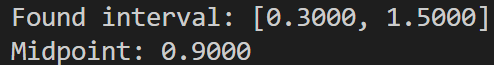
Results Display:

The program will output text results similar to the following:

At the same time, a visual chart will pop up:

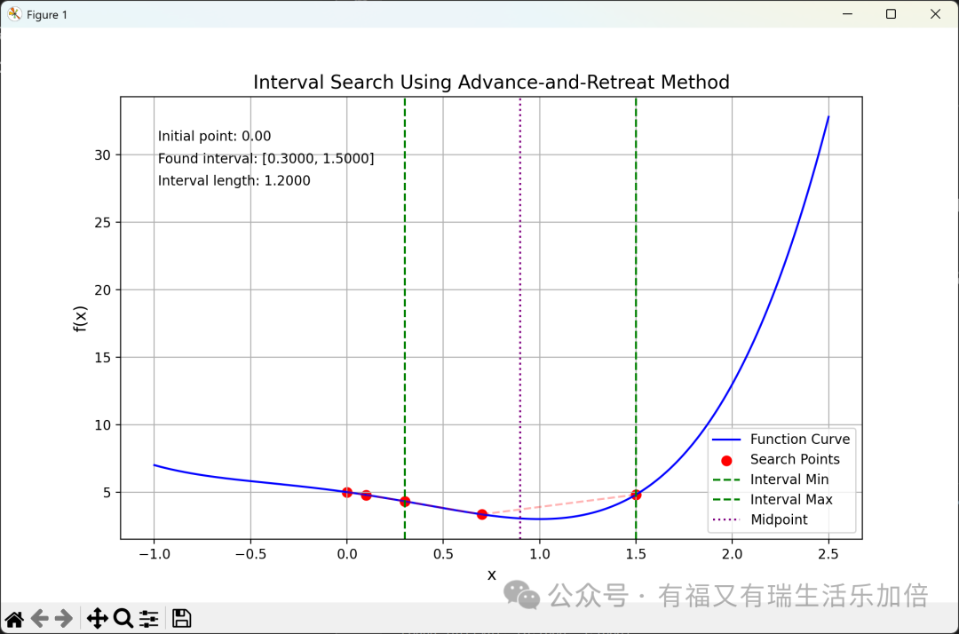
Result Interpretation:

From the output result <span>Found interval: [0.3000, 1.5000]</span> and the green dashed line marked in the chart, we can clearly know: For the function , the Advance-and-Retreat Method, starting from with as the initial step size, ultimately determined that one of its extremum points must be hidden within the interval [0.3, 1.5]!

Next Steps:

Now that we have successfully narrowed the infinite real number range down to a finite interval <span>[0.3, 1.5]</span>, we can confidently apply various more advanced one-dimensional search techniques (such as the Golden Section Method, Newton’s Method, etc.) to conduct fine searches within this interval, ultimately extracting the precise value that minimizes !

This concludes our exploration of the Advance-and-Retreat Method! Do you feel you have a clearer understanding of the first step in optimization problems? Although the Advance-and-Retreat Method is simple, it embodies the core idea of “trial-feedback-adjustment” in optimization algorithms and serves as the foundation for many complex algorithms.

If you found today’s content helpful, please don’t hesitate to give us a like 👍 and a follow 👀! Feel free to share ↗️ with more friends interested in optimization, algorithms, and programming!

Do you have any questions or thoughts about the Advance-and-Retreat Method, or optimization methods you are looking forward to learning about next (like the Golden Section Method? Newton’s Method?)? Come and leave a message in the comments to let us know! 👇

Thank you all for reading, and see you next time! Stay tuned for more optimization secrets! ✨