1) AI Data Compression

Problem:

Large language models (LLM) are powerful, but their massive scale and computational demands often present practical challenges. Deploying a model with billions of parameters requires substantial memory, processing power, and energy consumption, limiting their application in resource-constrained environments such as mobile devices or edge hardware, and increasing operational costs for cloud deployment.

Solution:

There are several compression methods:

lQuantization: Use low-precision numbers (e.g., 8-bit fixed-point instead of 32-bit floating-point) to represent model parameters/activations.

lPruning:: Identify and remove redundant or less important parameters (weights) or structures (such as entire neurons or channels) in the model.

·Unstructured pruning: Remove individual weights, resulting in a sparse matrix that requires specialized hardware or libraries for acceleration.

·Structured pruning: Remove larger, regular blocks of weights (e.g., entire channels or filters), making it easier to achieve acceleration on standard hardware.

lKnowledge Distillation: A smaller “student” model is trained to mimic the behavior of a larger pre-trained “teacher” model. The student model learns from the teacher model’s outputs (e.g., probability distributions over classes) or internal representations, effectively transferring knowledge to a more compact form.

lLow-Rank Decomposition: This method targets large weight matrices in the model (e.g., matrices in fully connected layers or attention layers). It approximates these matrices by decomposing them into products of smaller matrices, reducing the total number of parameters and associated computations. Techniques such as Singular Value Decomposition (SVD) are commonly used here.

These methods each have a range of trade-offs involving the degree of compression achieved, the impact on model accuracy, implementation complexity, and the inference acceleration achieved on different hardware platforms.

Quantization stands out, especially for large language models, as reducing numerical precision directly translates to lower memory bandwidth requirements (often a bottleneck) and can leverage highly optimized integer arithmetic operations on many modern CPUs and GPUs. It typically provides a good balance between compression ratio, performance improvement, and model accuracy retention.

2) Quantization:

The large and complex nature of AI models often makes them daunting, especially when it comes to limitations in computational resources and storage space. However, there is a magical technique—quantization, which acts like a magic wand, allowing models to become smaller, faster, and more energy-efficient without losing too much performance. From high-precision FP32 to low-precision INT4, what exactly is quantization?

Quantization is like turning a high-resolution painting into a low-resolution one while trying to keep it looking similar. In the world of computers, quantization refers to converting data in a model from high-precision representation to low-precision representation. For example, converting FP32 (32 bit floating-point) to FP16 (16 bit floating-point) or INT8 (8 bit integer).

2.1 Significance of Quantization

lLower memory usage: Lower precision means less memory is required for each parameter.

lIncreased speed: Integer operations are often much faster than floating-point operations (FlOps) especially on hardware optimized for low-bit computations.

lEnergy efficiency: Lower precision computations consume significantly less power, making them ideal for mobile and edge devices.

2.2 Types of Quantization

1)Uniform quantization: This method uniformly maps a range of floating-point values to integer values.

2)Non-uniform quantization: Uses a more complex mapping based onnetwork weights or activation distributions.

3)Symmetric and asymmetric quantization:

nSymmetric: Uses the same scale and zero point for both positive and negative values.

ØSigned INT8: Represents both positive and negative values. Its typical range is from-128 to 127. This is useful for representing weights or activation values, as they are often centered around zero.

ØSigned INT4: Typically represents values in the range of -8 to 7.

nAsymmetric: Allows different scales and zero points, which is useful for distributions that are not centered around zero.

ØUnsigned INT8: Represents only non-negative values. The range is from 0 to 255. Suitable for activation values that are always positive, such as those after a ReLU activation function, although signed integers are more common in weights.

ØUnsigned INT4: Represents values in the range of 0 to 15.

2.3 Linear Mapping Principle:

Maps the floating-point range [Rmin,Rmax] to the 8-bit integer range [0,255], the mapping may be as follows:

Converted (from original real valuer, to obtain the quantized valueq):

q= round(r/S) +Z

So the dequantization (from quantized valueq, to obtain the original real valuer):

r=s*(q-z)

Where,

SScale factor: Sets the step size between quantized values.Fixed-point numbers are essentially1 integer implicitly scaled by a preset factor. For example, you might decide to use a 8-bit signed integer (range from -128 to 127) to represent values between -1.0 and +1.0. To do this, you need to define a scaling factor of 2^7=128.

ZZero point: The integer value assigned to the real number zero.

2.4 Quantization Process

That is the conversion fromr toq involves dividing by the scale factor, adding the zero point, rounding to the nearest integer, and clamping the result to the allowed integer range (e.g.,INT8 is [-128, 127]):

q = clip(round(r / s) + z, q_min, q_max)

The scale factor (s) and zero point (z) define the quantization scheme, the two main schemes are symmetric quantization and asymmetric quantization.

2.4.1 Symmetric Quantization

· Mapping method:

It maps the floating-point range[−R, R] to the signed integer range[q_min, q_max], typically like INT8 as [−127, 127] or[−128, 127]. Its characteristic is that the floating-point value 0.0 directly maps to the integer value 0.

· Scale factor and zero point:

1.Zero point (z) is fixed at 0..

2.Scale factor (s) is determined by the maximum absolute value in the range you want to represent (R) Specifically,R = max(|min(r)|, |max(r)|) or simply for the entire tensor/channel/group as R = max(|r|). Then calculate the scale factor to map this maximum absolute valueR to the boundaries of the integer range. For mapping to[−127, 127] for signed INT8, the scale factor will be s = R / 127.

· Formula:

1.Quantization:q = clip(round(r/s), q_min, q_max) (zero point is 0)

2.Dequantization:r ≈ s*q

· Example:

Assuming quantizing values in the range [−3.8, 3.2] to signed INT8 (using [−127, 127] range for symmetric processing).

1.Determine the range limitR=max(|−3.8|,|3.2|) = 3.8

2.Calculate the scale factors=3.8/127 ≈ 0.0299

3.Set the zero pointz=0

4.Quantize a value, for exampler=1.5:q=round(1.5/0.0299) = round(50.167) = 50.

5.Quantize a value, for exampler=−0.8:q=round(−0.8/0.0299) = round(−26.75) = −27.

6.Dequantizeq=50:r≈0.0299*50=1.495.

7.Dequantizeq=−27:r≈0.0299*(−27)=−0.8073.

· Advantages:

1.Simplicity: The zero point is fixed at 0, simplifying calculations.

2.Efficiency: When the zero point is 0 , some hardware accelerators can perform integer calculations more efficiently.

· Disadvantages:

1.Potential inefficiency: If the original floating-point distribution is skewed (not centered around zero), one side of the integer range may be underutilized or unused, which can effectivelyreduce available precision.

2.4.2 Asymmetric Quantization

Asymmetric quantization maps the observed precise floating-point minimum and maximum values in the tensor to the minimum and maximum values of the integer range. This method is particularly useful when the data distribution is not centered around zero.

Mapping method

Maps the floating-point range[min(r),max(r)] to the full integer range [qmin,qmax], for example:

·Unsigned INT8 (UINT8) of [0,255]

·Signed INT8 of [−128,127].

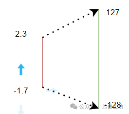
Scale factor and zero point

·Scale factor (s): Calculated based on the full floating-point range:s=(max(r)−min(r))/(qmax−qmin)

·Zero point (z): Ensures that the floating-point value 0.0 is correctly mapped to the quantized value, calculated as an integer offset:z=round(qmin−smin(r)/s)

Note::z may not be 0, it represents the integer value corresponding to the real number 0.0 In practice, the zero point is often clamped to the integer range [qmin,qmax], if clamping is needed, the scale factor may need to be adjusted.

Formula

·Quantization::q=clip(round(s/r)+z, qmin, qmax)

·Dequantization::r≈s*(q−z)

Example

Assuming quantizing activation values in the range[0.5,6.2] to unsigned INT8 (UINT8, range [0,255]):

1.Determine the range:min(r)=0.5, max(r)=6.2.

2.Calculate the scale factor s:s=255−6.2−0.5=255.7≈0.02235

3.Calculate the zero point z:z=round(0−0.022350.5)=round(−22.37)=−22

4.Quantize r=1.5:q=clip(round(0.022351.5)−22, 0, 255)=clip(67−22, 0, 255)=45

5.Quantize r=5.0:q=clip(round(0.022355.0)−22, 0, 255)=clip(224−22, 0, 255)=202

6.Dequantize q=45:r≈0.02235⋅(45−(−22))=0.02235⋅67≈1.497

7.Dequantize q=202:r≈0.02235⋅(202−(−22))=0.02235⋅224≈4.99

· Advantages:

Flexibility: Can accurately represent skewed or non-centered data distributions (e.g.,ReLU activation function outputs are always non-negative).

Precision: Maximizes the utilization of the integer range, providing lower quantization error for data with asymmetric distributions compared to symmetric quantization.

· Disadvantages:

Complexity: Dequantization and subsequent calculations require additional handling of the scale factor and zero point, introducing computational and storage overhead compared to symmetric quantization where the zero point is fixed at0..

2.5 Quantization Strategies:

Post-training quantization (PTQ) and quantization-aware training (QAT)

1) Post-training quantization (PTQ):

Quantization is performed on a model that has been trained using standard high-precision floating-point numbers (typicallyFP32).

PTQ is easier and faster to implement, but it may have a slightly larger drop in accuracy compared to QAT.

2)Quantization-aware training (QAT):

Instead of quantizing a fully trained model, it simulates low-precision behavior while the model weights are still being updated. The core idea is to insert operations into the model’s computation graph to simulate quantization and dequantization steps (FP32→INT8→FP32). These are often referred to as “fake quantization” nodes. During the forward pass of training, weights and/or activation values are quantized before being used for subsequent operations, and then immediately dequantized. This forces the model to learn parameters that can handle the noise and information loss introduced by the quantization process.

Integrating simulated quantization into the training process allows the model to adjust its weights based on quantization noise, achievinghigher accuracy..

—- The next section continues to introduce PTQ and QAT —-