Matlab EOF Analysis

%% EOF Analysis
clc;clear;close all

%% Read Precipitation Related Data
datadir = 'E:\prep\';
% Loop to read precipitation data
filelist=dir([datadir,'*.nc']);     
for  i = 1:129          
    ncid =[datadir,filelist(i).name];    
    time(:,i)=ncread(ncid,'time');    
    precip(:,:,i)=ncread(ncid,'precip');
end
path = [datadir,filelist(1).name];
ncdisp(path)
mlat = double(ncread(path,'latitude'));
mlon = double(ncread(path,'longitude'));
[nlat,nlon]=meshgrid(mlat,mlon);

%% Read shp Data
cdL=shaperead("E:\世界地图shp\世界地图2017\2017世界地图.shp");
cx=[cdL(:).X]; cy=[cdL(:).Y];

%% Calculation
precip=(reshape(precip,20*14,129))';     % Transform 3D data to 2D data

F=detrend(precip,0);                     % Remove mean (0th order polynomial trend)
C=F'*F;                                   % Calculate covariance matrix C

[EOFs,D]=eig(C);                         % EOF eigenvectors, D eigenvalues
PCs=EOFs'*F';                            % Time weights PC

D=diag(D);                                % Extract diagonal elements to get eigenvalue sequence
D=D./sum(D);                             % Standardize eigenvalues

%% First Mode
EOF1=EOFs(:,D==max(D));                  % Select the largest eigenvalue as the first mode
PC1=PCs(D==max(D),:);

EOF1=reshape(EOF1,20,14);                % Reshape to 20*14 spatial data

EOF1=EOF1.*std(PC1);                     % Standardize
PC1=PC1./std(PC1);
disp(max(D)*100)                         % Display variance explanation degree

%% Second Mode
EOF2=EOFs(:,279);                        % Select the second largest eigenvalue as the second mode
PC2=PCs(279,:);

EOF2=reshape(EOF2,20,14);

EOF2=EOF2.*std(PC2);
PC2=PC2./std(PC2);
disp(D(279,1)*100)

%% Plotting
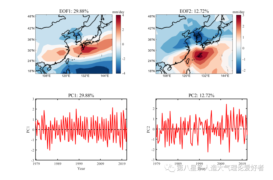
figure('position',[300,10,1200,800])

% First mode spatial distribution
subplot(2,2,1);
m_proj('miller','lon',[min(mlon) max(mlon)],'lat',[min(mlat) max(mlat)]);
m_contourf(nlon,nlat,EOF1,'linestyle','none');
m_grid('linestyle','none','xtick',([108 120 132 144]));
hold on
m_plot(cx,cy,'k','linewidth',2); 
colormap(m_colmap('diverging'));
s=colorbar('fontname','Times New Roman','fontsize',12);
title(s,'mm/day','fontname','Times New Roman');
set(gca,'fontsize',12)
title('EOF1: 29.88%','fontsize',16,'fontname','Times New Roman');

% First mode time series
subplot(2,2,3);
plot(1:129,PC1,'r','linewidth',2);
hold on
plot(xlim,[0,0],'k--','LineWidth',1.5)
set(gca,'xtick',[2:30:129],'xticklabels',1979:10:2021, ...
    'fontname','Times New Roman','fontsize',12);
xlabel('Year','fontname','Times New Roman');
ylabel('PC1','fontname','Times New Roman');
xlim([1 129]);
% ylim([-2.5 2.5]);
set(gca,'fontsize',12,'linewidth',2)
title('PC1: 29.88%','fontsize',16,'fontname','Times New Roman');

% Second mode spatial distribution
subplot(2,2,2);
m_proj('miller','lon',[min(mlon) max(mlon)],'lat',[min(mlat) max(mlat)]);
m_contourf(nlon,nlat,EOF2,'linestyle','none');
m_grid('linestyle','none','xtick',([108 120 132 144]));
hold on
m_plot(cx,cy,'k','linewidth',2); 
colormap(m_colmap('diverging'));
s=colorbar('fontname','Times New Roman','fontsize',12);
title(s,'mm/day','fontname','Times New Roman');
set(gca,'fontsize',12)
title('EOF2: 12.72%','fontsize',16,'fontname','Times New Roman');

% Second mode time series
subplot(2,2,4);
plot(1:129,PC2,'r','linewidth',2);
hold on
plot(xlim,[0,0],'k--','LineWidth',1.5)
set(gca,'xtick',[2:30:129],'xticklabels',1979:10:2021, ...
    'fontname','Times New Roman','fontsize',12);
xlabel('Year','fontname','Times New Roman');
ylabel('PC2','fontname','Times New Roman');
xlim([1 129]);
set(gca,'fontsize',12,'linewidth',2)
title('PC2: 12.72%','fontsize',16,'fontname','Times New Roman');