1. Environment Setup
The gym is a toolkit for developing and comparing reinforcement learning algorithms, and installing the gym library and its sub-environments in Python is quite straightforward.
Install gym:
pip install gym
Install the autonomous driving module, using the highway-env package published by Edouard Leurent on GitHub (link: https://github.com/eleurent/highway-env):
pip install --user git+https://github.com/eleurent/highway-env
This package includes six scenarios:
- Highway – “highway-v0”
- Merge – “merge-v0”
- Roundabout – “roundabout-v0”
- Parking – “parking-v0”
- Intersection – “intersection-v0”
- Racetrack – “racetrack-v0”
For detailed documentation, refer to:
https://highway-env.readthedocs.io/en/latest/
2. Environment Configuration
Once installed, you can conduct experiments in the code (taking the highway scenario as an example):
import gym
import highway_env
%matplotlib inline

env = gym.make('highway-v0')
env.reset()
for _ in range(3):
    action = env.action_type.actions_indexes["IDLE"]
    obs, reward, done, info = env.step(action)
    env.render()
After running, the following scene will be generated in the simulator:
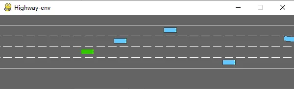
The green represents the ego vehicle. The env class has many parameters that can be configured; refer to the original documentation for specifics.
3. Training the Model
1. Data Processing
(1) State
The highway-env package does not define sensors; all vehicle states (observations) are read from the underlying code, saving a lot of initial workload. According to the documentation, states (observations) can be output in three ways: Kinematics, Grayscale Image, and Occupancy grid.
Kinematics
Outputs a matrix of V*F, where V represents the number of vehicles to observe (including the ego vehicle itself), and F represents the number of features to be counted. Example:

Data generation will default to normalization, with a value range of: [100, 100, 20, 20]. You can also set whether the attributes of vehicles other than the ego vehicle are absolute coordinates on the map or relative coordinates to the ego vehicle.
When defining the environment, you need to set the parameters for the features:
config = \
    {\
    "observation": \
         {\
        "type": "Kinematics",\
        # Select 5 vehicles for observation (including ego vehicle)\
        "vehicles_count": 5,  \
        # Total of 7 features\
        "features": ["presence", "x", "y", "vx", "vy", "cos_h", "sin_h"], \
        "features_range": \
            {\
            "x": [-100, 100],\
            "y": [-100, 100],\
            "vx": [-20, 20],\
            "vy": [-20, 20]\
            },\
        "absolute": False,\
        "order": "sorted"\
        },\
    "simulation_frequency": 8,  # [Hz]\
    "policy_frequency": 2,  # [Hz]\
    }
Grayscale Image
Generates a W*H grayscale image, where W represents the image width and H represents the image height.
Occupancy grid
Generates a WHF three-dimensional matrix, representing the vehicle situation around the ego vehicle in a W*H grid, with each cell containing F features.
(2) Action
The actions in the highway-env package are divided into continuous and discrete types. Continuous actions can directly define the values of throttle and steering angle, while discrete actions include 5 meta actions:
ACTIONS_ALL = {\
        0: 'LANE_LEFT',\
        1: 'IDLE',\
        2: 'LANE_RIGHT',\
        3: 'FASTER',\
        4: 'SLOWER'\
    }
(3) Reward
Except for the parking scenario, the highway-env package uses the same reward function:
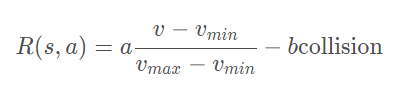
This function can only be modified in its source code; adjustments can only be made to the weights externally. (The reward function for the parking scenario is documented, but I won’t type out the formula…)
2. Building the Model
The structure and building process of the DQN network have been discussed in another article of mine, so I won’t elaborate here. I will demonstrate using the first state representation method – Kinematics.
Since the state data volume is small (5 vehicles * 7 features), CNN can be disregarded, and the two-dimensional data size [5,7] can be directly converted to [1,35]. Thus, the model input is 35, and the output is the number of discrete actions, which is 5.
import torch
import torch.nn as nn
from torch.autograd import Variable
import torch.nn.functional as F
import torch.optim as optim
import torchvision.transforms as T
from torch import FloatTensor, LongTensor, ByteTensor
from collections import namedtuple
import random
Tensor = FloatTensor

EPSILON = 0    # epsilon used for epsilon greedy approach
GAMMA = 0.9
TARGET_NETWORK_REPLACE_FREQ = 40       # How frequently target network updates
MEMORY_CAPACITY = 100
BATCH_SIZE = 80
LR = 0.01         # learning rate

class DQNNet(nn.Module):
    def __init__(self):
        super(DQNNet,self).__init__()
        self.linear1 = nn.Linear(35,35)
        self.linear2 = nn.Linear(35,5)
    def forward(self,s):
        s=torch.FloatTensor(s)
        s = s.view(s.size(0),1,35)
        s = self.linear1(s)
        s = self.linear2(s)
        return s

class DQN(object):
    def __init__(self):
        self.net,self.target_net = DQNNet(),DQNNet()
        self.learn_step_counter = 0
        self.memory = []
        self.position = 0
        self.capacity = MEMORY_CAPACITY
        self.optimizer = torch.optim.Adam(self.net.parameters(), lr=LR)
        self.loss_func = nn.MSELoss()

    def choose_action(self,s,e):
        x=np.expand_dims(s, axis=0)
        if np.random.uniform() < 1-e:
            actions_value = self.net.forward(x)
            action = torch.max(actions_value,-1)[1].data.numpy()
            action = action.max()
        else:
            action = np.random.randint(0, 5)
        return action

    def push_memory(self, s, a, r, s_):
        if len(self.memory) < self.capacity:
            self.memory.append(None)
        self.memory[self.position] = Transition(torch.unsqueeze(torch.FloatTensor(s), 0),torch.unsqueeze(torch.FloatTensor(s_), 0),\
                                                torch.from_numpy(np.array([a])),torch.from_numpy(np.array([r],dtype='float32')))#
        self.position = (self.position + 1) % self.capacity

    def get_sample(self,batch_size):
        sample = random.sample(self.memory,batch_size)
        return sample

    def learn(self):
        if self.learn_step_counter % TARGET_NETWORK_REPLACE_FREQ == 0:
            self.target_net.load_state_dict(self.net.state_dict())
        self.learn_step_counter += 1

        transitions = self.get_sample(BATCH_SIZE)
        batch = Transition(*zip(*transitions))

        b_s = Variable(torch.cat(batch.state))
        b_s_ = Variable(torch.cat(batch.next_state))
        b_a = Variable(torch.cat(batch.action))
        b_r = Variable(torch.cat(batch.reward))

        q_eval = self.net.forward(b_s).squeeze(1).gather(1,b_a.unsqueeze(1).to(torch.int64))
        q_next = self.target_net.forward(b_s_).detach() #
        q_target = b_r + GAMMA * q_next.squeeze(1).max(1)[0].view(BATCH_SIZE, 1).t()
        loss = self.loss_func(q_eval, q_target.t())
        self.optimizer.zero_grad() # reset the gradient to zero
        loss.backward()
        self.optimizer.step() # execute back propagation for one step
        return loss
Transition = namedtuple('Transition',('state', 'next_state','action', 'reward'))
3. Running Results
Once all parts are completed, you can combine them to train the model. The process is similar to using CARLA, so I won’t go into detail.
Initialize the environment (just add the DQN class):
import gym
import highway_env
from matplotlib import pyplot as plt
import numpy as np
import time
config = \
    {\
    "observation": \
         {\
        "type": "Kinematics",\
        "vehicles_count": 5,\
        "features": ["presence", "x", "y", "vx", "vy", "cos_h", "sin_h"],\
        "features_range": \
            {\
            "x": [-100, 100],\
            "y": [-100, 100],\
            "vx": [-20, 20],\
            "vy": [-20, 20]\
            },\
        "absolute": False,\
        "order": "sorted"\
        },\
    "simulation_frequency": 8,  # [Hz]\
    "policy_frequency": 2,  # [Hz]\
    }

env = gym.make("highway-v0")
env.configure(config)
Train the model:
dqn=DQN()
count=0

reward=[]
avg_reward=0
all_reward=[]

time_=[]
all_time=[]

collision_his=[]
all_collision=[]
while True:
    done = False
    start_time=time.time()
    s = env.reset()

    while not done:
        e = np.exp(-count/300)  # Probability of randomly selecting an action, gradually decreases as training progresses
        a = dqn.choose_action(s,e)
        s_, r, done, info = env.step(a)
        env.render()

        dqn.push_memory(s, a, r, s_)

        if ((dqn.position !=0)&&(dqn.position % 99==0)):
            loss_=dqn.learn()
            count+=1
            print('trained times:',count)
            if (count%40==0):
                avg_reward=np.mean(reward)
                avg_time=np.mean(time_)
                collision_rate=np.mean(collision_his)

                all_reward.append(avg_reward)
                all_time.append(avg_time)
                all_collision.append(collision_rate)

                plt.plot(all_reward)
                plt.show()
                plt.plot(all_time)
                plt.show()
                plt.plot(all_collision)
                plt.show()

                reward=[]
                time_=[]
                collision_his=[]

        s = s_
        reward.append(r)

    end_time=time.time()
    episode_time=end_time-start_time
    time_.append(episode_time)

    is_collision=1 if info['crashed']==True else 0
    collision_his.append(is_collision)
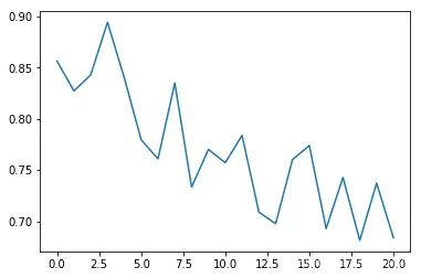
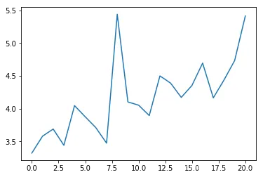
I added some plotting functions in the code, allowing you to monitor key metrics during the run, with averages calculated every 40 training iterations.
Average collision rate:
Average epoch duration (s):
Average reward:
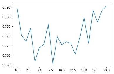
It can be seen that the average collision rate decreases as the number of training iterations increases, and the duration of each epoch gradually extends (if a collision occurs, the epoch ends immediately).
4. Conclusion
Compared to the simulator CARLA I used in previous articles, the highway-env environment package is clearly more abstract, using a game-like representation that allows algorithms to be trained in an ideal virtual environment without considering data acquisition methods, sensor accuracy, computation time, and other real-world issues. It is very friendly for end-to-end algorithm design and testing, but from the perspective of automatic control, there are fewer aspects to explore, making research less flexible.