Embedded AI Series – Code Analysis of YOLOv3 Deployment on RV1126 – Post-Processing 1

★

Embedded AI Series – Code Analysis of YOLOv3 Deployment on RV1126 – Post-Processing 1

”

1. Introduction

After executing inference and obtaining the inference results in the previous article, the next step is to parse and process the inference results, commonly referred to as “post-processing.” The knowledge points involved in the post-processing section are quite extensive and will be divided into several articles for introduction.

PS: The complete code for this article can be found in “Embedded AI Series – Deploying YOLOv3 Model on RV1126”

2. Querying Output Information of RKNN Model

The previous article “Embedded AI Series – Code Analysis of YOLOv3 Deployment on RV1126 – Model Input Information” introduced how to query the number of input and output tensors of the RKNN model and how to query input attribute information.

Using a similar method, you can call rknn_query with the parameter RKNN_QUERY_OUTPUT_ATTR to obtain the output attribute information of the model. The code snippet is as follows:

// io_num.n_output is 3
rknn_tensor_attr output_attrs[io_num.n_output];
memset(output_attrs, 0, sizeof(output_attrs));
for (int i = 0; i < io_num.n_output; i++) {
    output_attrs[i].index = i;
    ret = rknn_query(ctx, RKNN_QUERY_OUTPUT_ATTR, &(output_attrs[i]), sizeof(rknn_tensor_attr));
    if (ret < 0) {
        printf("rknn_query output_attr error ret=%d\n", ret);
        rknn_destroy(ctx);
        return -1;
    }
    dump_tensor_attr(&(output_attrs[i]));
    // Validate output size
    if (output_attrs[i].dims[2] != ANCHOR_PER_LAYER * (NUM_CLASSES + 5)) {
        std::cerr << "Warning: Output channels mismatch! Expected: " << ANCHOR_PER_LAYER * (NUM_CLASSES + 5) << ", Actual: " << output_attrs[i].dims[2] << std::endl;
    }
}

From the actual printout, we can see the information of the 3 model output tensors:

3. Why Does the YOLOv3 Model Have 3 Tensor Outputs?

In traditional object detection methods, multiple scans of the image are required for analysis, while YOLO only needs to scan once, i.e., “one forward pass,” to complete the object detection task, which is the origin of its name YOLO (You Only Look Once).

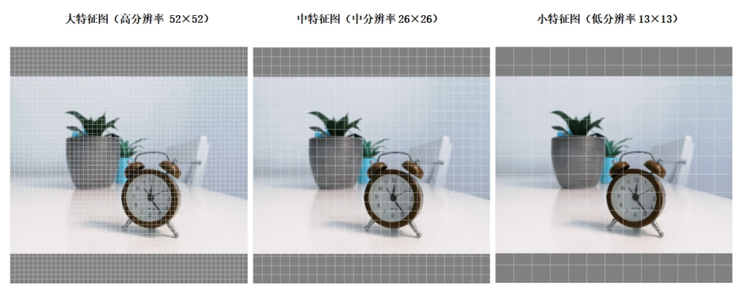
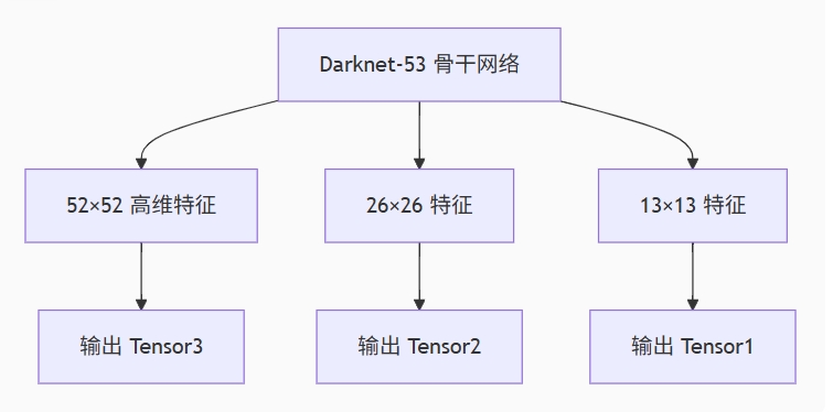
To better detect objects of different sizes, the internal network structure of YOLOv3 uses 3 feature maps of different scales (13×13, 26×26, 52×52) for predictions:

• Large feature map (high resolution, 52×52): small receptive field, suitable for detecting small objects (e.g., distant pedestrians, small animals)
• Medium feature map (medium resolution, 26×26): suitable for detecting medium objects (e.g., cars, bicycles)
• Small feature map (low resolution, 13×13): large receptive field, suitable for detecting large objects (e.g., buses, buildings)

In simple terms, the input image of 416 * 416 is divided into 3 different sizes of grids for processing, as shown in the figure:

4. Data Parsing of Each Output Tensor of YOLOv3 Model

Taking the first output tensor as an example, the printout is:

“index=0,name=output_82_199,n_dims=4,dims=[1, 255, 13, 13],n_elems=43095,size=43095,fmt=NCHW, type=UINT8,qnt_type=AFFINE,zp=182,scale=0.123265”.

(Note: The current format is NCHW, but the order stored in output_attrs’ dims is reversed (WHCN), i.e., dims[0] is width, dims[1] is height, dims[2] is the number of channels, dims[3] is batch size)

It can be seen that output tensor 1 has 255 channels, with each channel corresponding to a 13 * 13 matrix of data. In other words, each grid cell in the 13 * 13 grid matrix corresponds to the data information of 255 channels.

4.1 Why Are There 255 Channels?

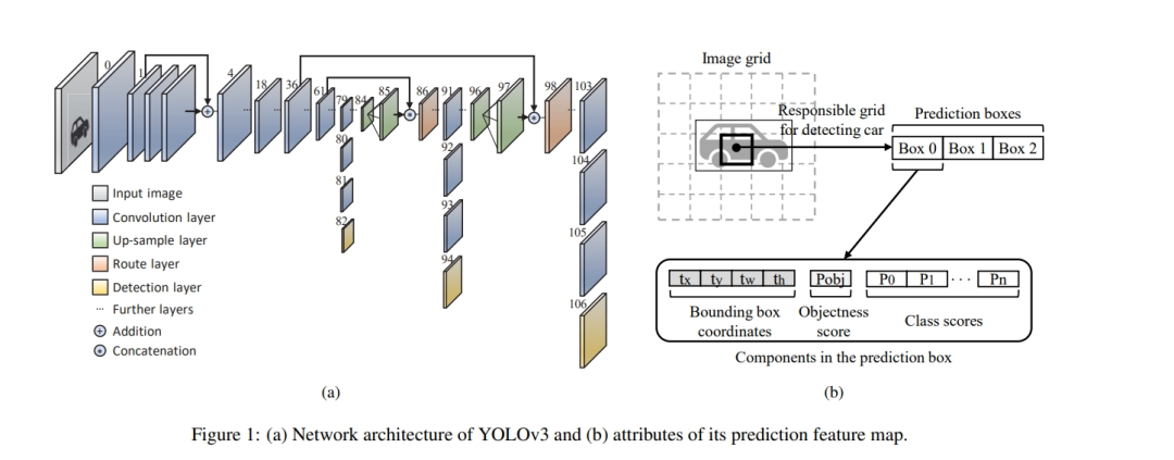
Image source:

https://openaccess.thecvf.com/content_ICCV_2019/papers/Choi_Gaussian_YOLOv3_An_Accurate_and_Fast_Object_Detector_Using_Localization_ICCV_2019_paper.pdf

As shown in the above figure (b), each grid cell in the output feature map grid matrix (Image grid) corresponds to a predicted object, containing three prediction boxes (Prediction boxes). Each prediction box’s information includes 4 target coordinate values (tx, ty, tw, th), 1 object confidence score (i.e., likelihood), and 80 class confidence scores (YOLOv3 can predict 80 types, and the likelihood of each type will be output separately), meaning that the information contained in a predicted object is 3 * (4 + 1 + 80) = 255.

4.2 Memory Layout of Model Output Data

For each spatial position (h, w) on the output feature map (corresponding to a grid area on the original image), 255 values are stored contiguously in memory. These 255 values (the aforementioned 255 channels) are arranged in the following order:

• 85 values for the first predicted bounding box (bbox0):

  [0]: tx or x (center point x offset)

  [1]: ty or y (center point y offset)

  [2]: tw or w (width scale)

  [3]: th or h (height scale)

  [4]: objectness score (object confidence)

  [5] to [84]: 80 class probabilities (class probabilities)

• 85 values for the second predicted bounding box (bbox1):

  [85] – [169] (same structure as above)

• 85 values for the third predicted bounding box (bbox2):

  [170] – [254] (same structure as above)

Therefore, the values at (n=0, c, h, w) in memory are:

c=0 -> bbox0’s tx

c=1 -> bbox0’s ty

…

c=4 -> bbox0’s objectness

c=5 -> bbox0’s class0 probability

…

c=84 -> bbox0’s class79 probability

c=85 -> bbox1’s tx

… and so on

4.3 What Are Predefined Anchor Boxes?

The coordinates of the three predicted boxes mentioned above are derived from predefined anchor boxes. In the subsequent code explanation, you will see how the coordinates of the predicted boxes and anchor boxes are used to calculate the actual coordinates of the target.

The concept of predefined anchor boxes introduced by YOLOv3 is one of its core innovations.

Predefined anchor boxes are a set of fixed-width and height boxes that cover the most common aspect ratios. During the model’s internal inference predictions, this set of anchor boxes is tiled across the image, allowing the model to reference these predefined anchor boxes to assist in locating the detection targets, making the localization process faster and more efficient.

Different anchor boxes use different aspect ratios, suitable for different targets:

Anchor Box Type	Typical Aspect Ratio	Suitable Targets
Anchor Box 1	1:3	Standing people/animals
Anchor Box 2	3:1	Cars/boats, etc.
Anchor Box 3	1:1	Traffic lights/faces, etc.

For example:

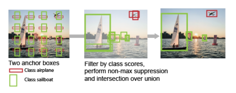
Image source:

https://www.mathworks.com/help/vision/ug/anchor-boxes-for-object-detection.html

• In the above image, there are two anchor boxes: 1. The red box is flat, suitable for locating airplanes; 2. The green box is tall and thin, suitable for locating sailboats.
• The first small image shows how the model internally tiles the two anchor boxes;
• The second small image in the middle shows the detection results stored in the model output tensor;
• The third small image on the right shows the final effect after our user code performs “Non-Maximum Suppression (NMS)” on the model output results to filter out duplicate detection boxes.

The detailed principles are not crucial for us AI application engineers; if interested, you can read more at: https://www.mathworks.com/help/vision/ug/anchor-boxes-for-object-detection.html

4.4 Why Does a Predicted Object Result Have 3 Prediction Anchor Boxes?

If there are more anchor boxes, it can improve recall but increase computation, as more parameters need to be predicted for each position;

If there are fewer anchor boxes, it will reduce the model’s expressive capability, increasing the missed detection rate;

Therefore, setting the number of predicted anchor boxes to 3 is a value that has been experimentally verified to achieve the best balance between model capacity and efficiency.