Skip to content
Abstract: When the wall has not moved enough to reach active or passive states, the intermediate earth pressure acts on the wall. These pressures are crucial for the design of embedded retaining walls; embedded walls are flexible structures that may experience different soil states along their length. Recently, the author proposed a continuous medium mechanics method to derive the earth pressure coefficient for any soil state between static and active or passive conditions, applicable to cohesive-friction soils and horizontal and vertical pseudo-static conditions. The same method also provides analytical expressions to calculate the required wall movement (at any depth) to achieve active or passive failure states. The author suggests combining this method with elastic beam theory to propose a new fully analytical method for designing embedded retaining walls. An application example is provided and compared with finite element methods.
When the wall has not moved enough to reach active or passive states, the intermediate earth pressure acts on the wall. These pressures are crucial for the design of embedded retaining walls; embedded walls are flexible structures that may experience different soil states along their length. The methods included in the standards should reflect best (current) practices. In 2001, BS 8002 [1] outlined five ‘traditional’ methods for designing embedded retaining walls, but mentioned that all these methods have significant flaws and limited applicability. These methods include: a) total pressure method, b) net available resistance method, c) strength factor method, d) net pressure method, and e) end-fixity method. Newer EN1997-1:2004 [2] and prEN1997-3:2022 [3] (draft standards) recommend using empirical rules (such as interpolation), spring models, or continuous numerical models to calculate intermediate values of intermediate earth pressure. However, spring models also heavily rely on empirical rules to determine the spring constant. Clearly, the simplicity and empirical nature of the above methods raise serious doubts about their effectiveness. Therefore, among the various methods mentioned above, numerical simulation seems to be the best choice. However, intermediate earth pressure highly depends on the initial stresses set in the program; these initial stresses are not always correctly defined for cohesive or over-consolidated soils. On the other side of the ocean (e.g., [4, 5]), the situation seems to be similar. This paper aims to propose a reliable design method for embedded retaining walls. The new method is based on the generalized earth pressure coefficient theory recently proposed by the author [6], combined with static elastic beam theory.
Generalized Earth Pressure Coefficient
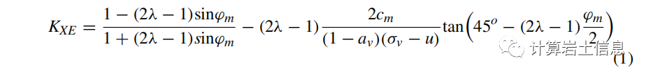
In 2019, the author [6] derived the earth pressure coefficient for any soil state between static and active or passive states through continuum mechanics, applicable to cohesive-friction soils and horizontal and vertical pseudo-static conditions. The basic earth pressure coefficient expression is:
For specific derivation processes, refer to – An Analytical Method for Designing Embedded Retaining Walls
Modern centrifuge tests and finite element analyses validating Pantelidis’ [6] continuum mechanics method can be found in Pantelidis and Christodoulou [7]. The above formula will be used to introduce a new method for designing embedded retaining walls.
Application Example and Numerical Validation
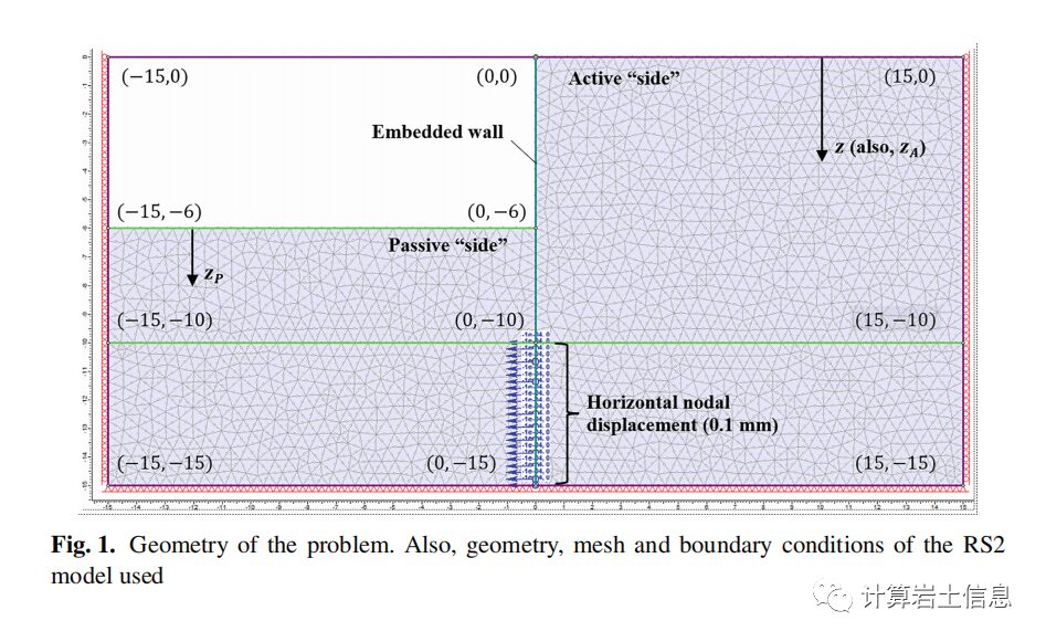
The following analysis combines the earth pressure method proposed by the author [6] and elastic beam theory (simple cantilever beam). The example shown in this paper has been solved using the KWall v.1 educational software prepared by the author and Dr. Panagiotis Christodoulou, as well as Rocscience’s RS2 (for validation purposes). The geometry, mesh, and boundary conditions of the problem are shown in Figure 1. The wall can freely bend from z = 0 to 10 meters, while below the depth point z = 10 meters, the wall is essentially fixed. During the analysis, it is assumed that both translation and rotation motion components are zero. In the numerical calculation process, wall anchoring is achieved by setting the horizontal node displacement to as low as 0.1 mm between z = 10 to 15 meters. This very small node displacement is applied within a five-meter height range below the wall instead of using a very stiff soil layer to obtain more stable results. The wall has a bending stiffness EW IW = 1.5GPa·m4, acting in a homogeneous, isotropic mass where the cohesion c‘= 0 kPa, internal friction angle ϕ’=30°, unit weight γ=20kN/m3, Young’s modulus E=20MPa, and Poisson’s ratio ν=0.3. To simplify, pore water pressure and seismic excitation are ignored.
To re-illustrate the problem, all relevant information is provided below (if not mentioned, RS2 default values are used). The solver type is set to ‘Gaussian elimination’. Regarding the ‘stress analysis’ menu, the maximum number of iterations is set to 1000, with a tolerance of 0.001, adopting ‘full convergence’ type. The ‘mesh type’ is set to ‘graded’, using 6-node triangular elements (i.e., 19.0 nodes or 9.2 elements per square meter; see Figure 1). The ‘field stress type’ is ‘gravity’, with the stress ratio of the internal and external planes equal to 0.5 (referring to the equations considered in soil at x = 0 m and aH = aV = 0). The initial loading method for the elements is ‘field stress and body force’. The problem is statically solved (aH = aV = 0). The soil parameters are the same as previously provided (the ‘plastic material’ type is evidently selected). The wall is modeled as a ‘structural interface’, where the line part is a ‘standard beam’ element with a ‘joint’ element on both sides. The lining is considered elastic, with Young’s modulus Ew=15·10^6 kPa and thickness of 1.0627 meters (moment of inertia Iw=1.06273·1/12= 0.1m4); this combination yields the value EwIw=1.5·106 kPa·m4 (beam stiffness) used by the author in the analytical solution (the lining’s Poisson’s ratio is 0.01, adopting the ‘Timoshenko’ beam element formula). Regarding the ‘joint’, the ‘material-related’ slip criterion is selected, and the ‘interface coefficient’ is set very low, only 0.05 (reminding that this earth pressure analysis method is suitable for smooth walls). The normal and shear stiffness of the joint element are both set to 200 MPa/m.
Regarding the proposed analysis process, the deflection y at any depth z is calculated based on elastic beam theory, where the embedded wall in Figure 1 is considered a cantilever beam; the earth pressure acting on both sides of the wall constitutes the load on the beam, using the superposition principle. An iterative process is required. As a starting point (first iteration), it is logical and convenient to assume that the soil on both sides of the wall is in a static state (i.e., y = 0 m, indicating the application of equation 1 for m = 1). However, since HA > HP, this state cannot be established at most points along the wall; the embedded wall will tend to bend towards the active ‘side’ (to some extent controlled by the wall’s bending stiffness). The total deflection yt of the wall caused by the earth pressure distribution acting on both sides is then calculated. For the second iteration, these total yt values become the x data values, and so on, until convergence is achieved. Performing five iterations is sufficient to obtain stable results. The final results are shown in Figures 2 and 3, obtained in the last (fifth) iteration and presented in graphical form.
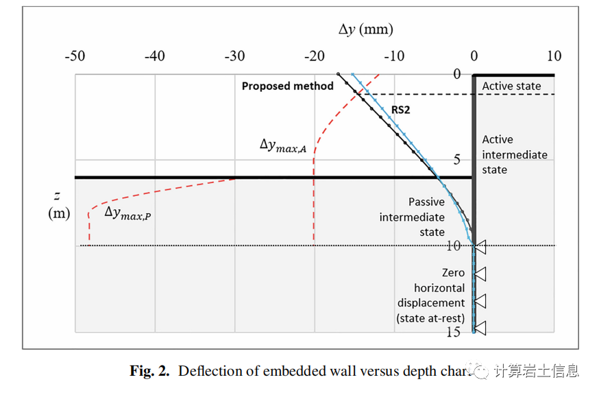
In the chart of Figure 2, the relationship between the analytical and numerically derived deflection values of the wall and depth has been plotted; simultaneously, the maximum deflection values under active and passive states (ymax,A and ymax,P respectively) are also shown on the same chart. In this regard, the following observations can be made: a) The proposed method effectively calculates the deflection of the embedded wall; b) There exists an active failure zone near the top of the wall (ytot ≥ ymax,A), while the soil near the remaining mass of the wall is in an intermediate active or passive state; c) The analytical solution indicates that the soil on the passive ‘side’ of the problem is far from reaching failure state; moreover, a deflection of only 4.5 mm (maximum deflection, referring to zP = 0 m) is insufficient to cause the specific soil to undergo active failure, let alone passive conditions.
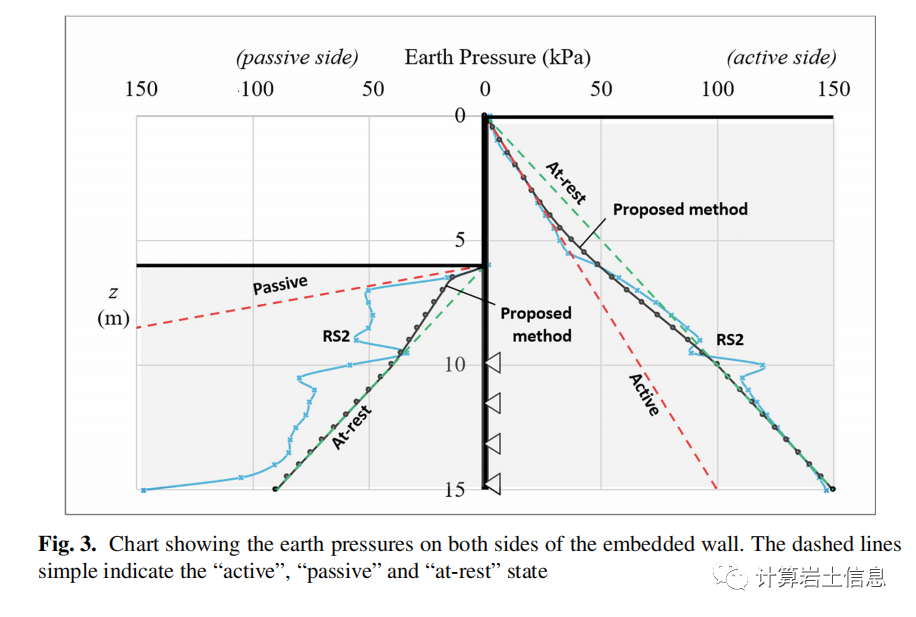
In Figure 3, the analytical and numerical earth pressure distribution corresponding to depth has been plotted. As shown, the ‘active’ curves (analytical and numerical) match very well. At the same time, as expected, for z > 10 m (i.e., below the theoretical fixed point of the wall), both curves are consistent with the earth pressure distribution under theoretical static conditions. For the passive state, the analytical curve shows earth pressure close to that under the corresponding static state, which can be demonstrated by the comparatively small deflection value of ymax,P threshold. On the other hand, the ‘passive’ numerical curve exhibits very peculiar behavior, with significantly high intermediate earth pressure values; in fact, in the range of 6m < z < 7m (0m ≤ zP ≤ 1m), they are very close to earth pressure under passive conditions. Moreover, at z > 10 m, the numerical earth pressure is much greater than the logically expected earth pressure under static conditions while the wall remains almost unchanged. Clearly, the static earth pressure on the ‘active’ side should also represent that on the ‘passive’ side; this difference is caused by the numerical process, which the author cannot explain.
The knowledge of intermediate earth pressure (i.e., the earth pressure between soil static state and active or passive states) is very important in designing embedded retaining structures. However, in the absence of reliable methods to compute these pressures (which depend on the degree of movement and bending of the flexible wall), global design standards rely on simplified methods, mainly assumptions, empirical rules, and parameters. To date, addressing the issue of intermediate earth pressure has been a ‘necessary evil’, the reliability of which is often disputed.
This paper proposes a new fully analytical method for designing embedded retaining walls. This combines the earth pressure theory proposed by the author in 2019 with elastic beam theory. An application example is given, showing significant consistency with finite element methods. The effectiveness of the proposed method involves not only the calculation of earth pressures but also the calculation of wall deflection profiles. Comparison with finite element methods shows excellent consistency. In fact, the proposed method has a tremendous advantage in terms of result stability compared to finite elements.
Finally, given the rationality and effectiveness of the proposed method, it can replace existing rough and semi-empirical methods, which not only lack a solid theoretical basis but also lack thorough calibration, leading to more cost-effective and reliable structures.