Video Explanation: Rolling Prediction of SPX Index Financial Time Series Volatility Using LSTM and GARCH

Full text link:https://tecdat.cn/?p=37371

This article integrates various technologies, among which the LSTM (Long Short-Term Memory) and GARCH (Generalized Autoregressive Conditional Heteroskedasticity) models are particularly crucial. LSTM excels in handling time series data, capturing long-term dependencies, and providing strong support for financial predictions. The GARCH model effectively captures the phenomenon of volatility clustering in financial time series, enhancing prediction accuracy.(Click “Read the original text” at the end for completecode data).

Video

Through a detailed interpretation and analysis of this code, including an in-depth discussion of key models such as LSTM and GARCH, we aim to inject new vitality into financial research and practice, opening up new ideas.

Introduction

In today’s complex and ever-changing financial market environment, in-depth data analysis and precise model construction are crucial for understanding market dynamics, predicting price trends, and formulating effective investment strategies.

Innovations

1. Integration of multiple advanced models: This approach combines the advantages of GARCH and LSTM models, integrating traditional financial models with deep learning methods, providing a more comprehensive and accurate means for financial data analysis and prediction.

2. Refined feature engineering: By calculating logarithmic returns and the volatility of the past 10 days, we delve into the potential information within financial data, improving the quality of model inputs and prediction performance.

3. Flexible data processing: Including operations such as transposing data, resetting indices, and handling missing values, this approach can adapt to different structures and qualities of financial data, enhancing its versatility and practicality.

Code Content and Analysis

Importing Required Libraries

import pandas as pd
from pandas.plotting import autocorrelation_plot
from pandas_datareader import data
import numpy as np
import matplotlib.pyplot as plt
import seaborn as sns
import math

The rich and powerful library imports lay a solid foundation for subsequent data processing and analysis. The Pandas library is used for data reading and manipulation, while Matplotlib and Seaborn are used for data visualization. Numpy provides efficient numerical computation support, and the Math library is used for mathematical operations.

Reading Financial Data from CSV File

df = pd.read_csv(r'inpv')
print(df.head())
print(df.shape)

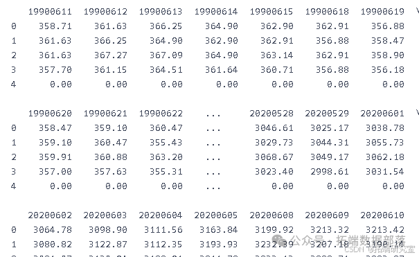
This part of the code reads financial data from a CSV file and prints the head and shape of the data to gain an initial understanding of its structure and scale.

Here we can see that we have 254 columns corresponding to 254 working days of financial data, along with 10 columns representing the 10 financial indicators we possess.

Data Cleaning

Transposing DataFrame Since we are dealing with time series data, we should treat the date as a column, so we use the transpose function.

df = df.transpose()
print(df.head())
print(df.shape)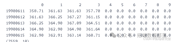

The transposition operation helps organize the data in a more suitable manner for subsequent analysis.

Resetting DataFrame Index

df = df.reset_index()
print(df.head())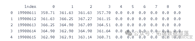

Resetting the index ensures that the data’s index is consistent and accurate.

import pandas as pd
import matplotlib.pyplot as plt
# Load data
file_path ='/mnt/data/financial_dataaned.csv'
df = pd.read_csv(file_path)
# Display the first few rows of the data to understand its structure
df.head()

The data has been successfully loaded. Next, I will conduct the following analyses and visualizations:

1. Trend chart of stock opening price, closing price, highest price, and lowest price.

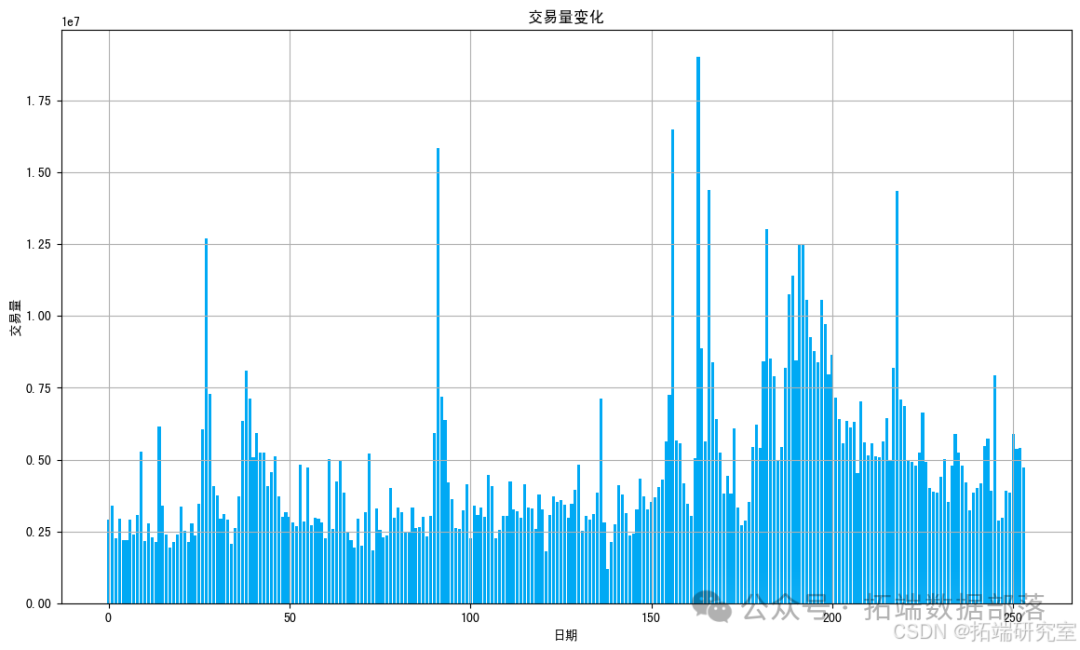
2. Trend chart of trading volume changes.

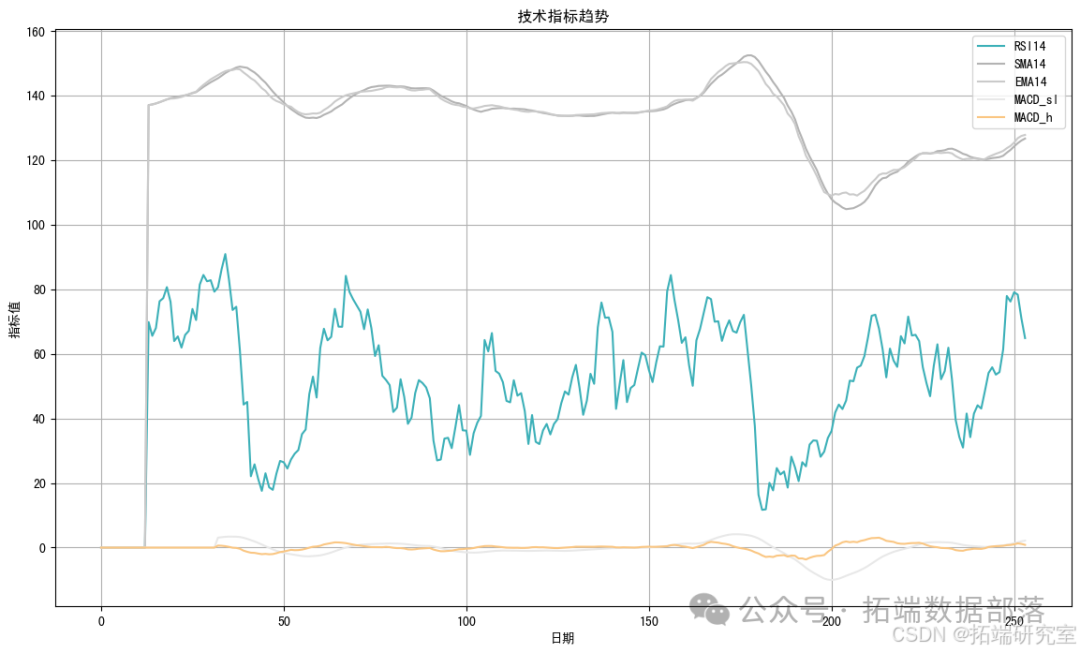
3. Trend chart of technical indicators (RSI14, SMA14, EMA14, MACD_sl, MACD_h).

Let’s start plotting the charts.

## Plotting the trend chart of stock opening price, closing price, highest price, and lowest price
plt.figure(figsize=(14,8))
plt.plot(df['Open'], color=colors[1], label='Opening Price')
plt.plot(df['Close'], color=colors[2], label='Closing Price')
plt.plot(df['High'], color=colors[3], label='Highest Price')
plt.plot(df['Low'], color=colors[4], label='Lowest Price')
plt.title('Stock Price Trend')
plt.xlabel('Date')
plt.ylabel('Price')
plt.legend()
plt.grid(True)
plt.show()
# Plotting the trend chart of trading volume changes
plt.figure(figsize=(14,8))
plt.bar(df.index, df['Volume'], color=colors[5])
plt.title('Trading Volume Changes')
plt.xlabel('Date')
plt.ylabel('Volume')
plt.grid(True)
plt.show()
# Plotting the trend chart of technical indicators
indicators = ['RSI14','SMA14','EMA14','MACD_sl','MACD_h']
plt.figure(figsize=(14,8))
for i, indicator in enumerate(indicators):
    plt.plot(df[indicator], color=colors[i + 6], label=indicator)
plt.title('Technical Indicators Trend')
plt.xlabel('Date')
plt.ylabel('Indicator Value')
plt.legend()
plt.grid(True)
plt.show()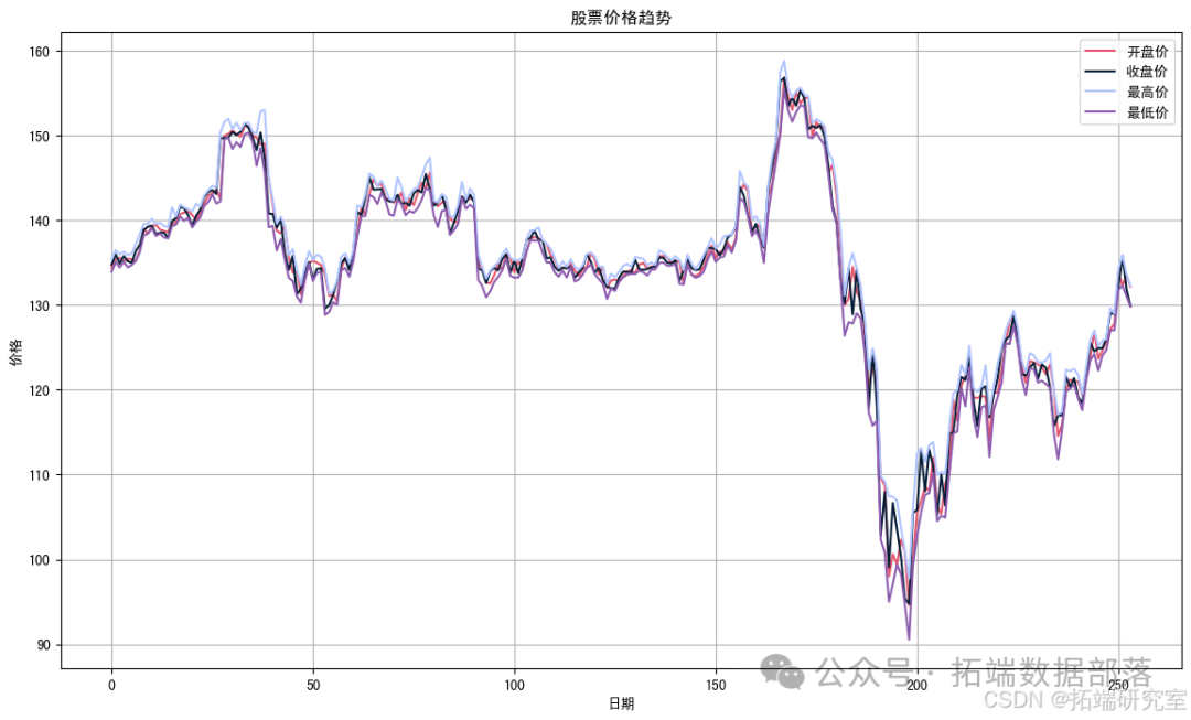

1. The first chart shows the trend of stock opening price, closing price, highest price, and lowest price.

2. The second chart displays the trend of trading volume changes.

3. The third chart illustrates the trend of technical indicators (RSI14, SMA14, EMA14, MACD_sl, MACD_h).

Click the title to check past content

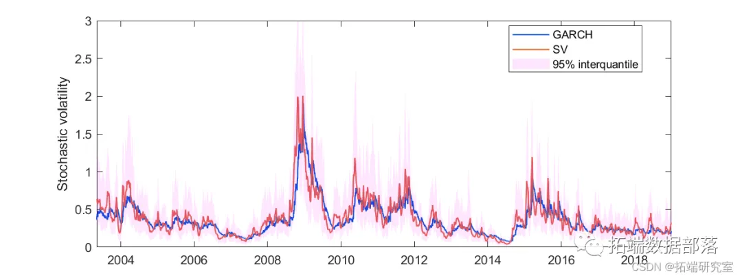
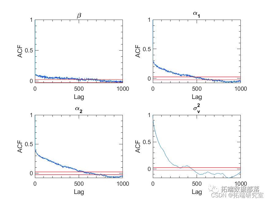
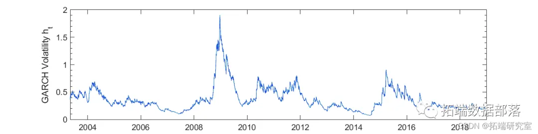
MATLAB Random Volatility SV, GARCH Analysis of Exchange Rate Time Series Using MCMC Markov Chain Monte Carlo Method

Swipe left to see more

01

02

03

04

Feature Engineering

Log Features – Log Returns

df['Log_Returns'] = np.log(df.Close) - np.log(df.Close.shift(1))
print(df.head())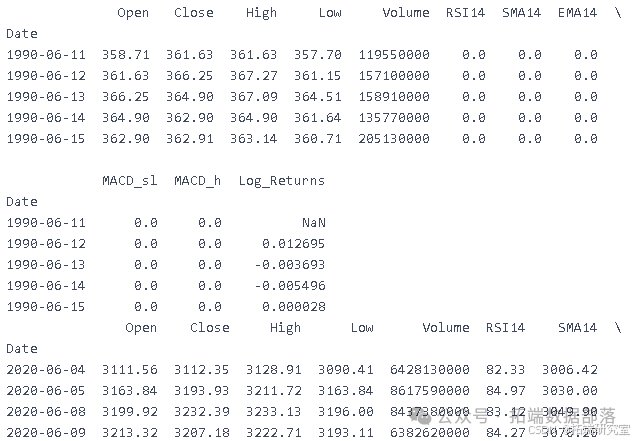

By calculating log returns, we can better capture the changing characteristics of financial data.

Volatility – Previous 10 Days’ Volatility

df['Previous_10_Day_Volatility'] = df['Log_Returns'].rolling(window=10).std()
print(df.tail())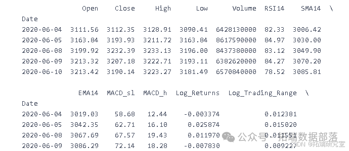

The calculation of volatility is significant for assessing the risk of financial assets.

GARCH

GARCH Prediction for the Entire SPX Dataset

Constructing a New DataFrame to Split Data into Test and Training Sets

X = df[df.first_valid_index():df.last_valid_index() - datetime.timedelta(1500)]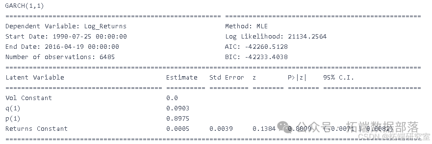

Using GARCH Model for Rolling Prediction

GARCH_rolling_predictions = GARCH_model.predict_is(h=len(X)-50, fit_once=True)

The GARCH model can capture the phenomenon of volatility clustering in financial time series data, improving prediction accuracy.

Constructing a New DataFrame to Split Data into Test and Training Sets

Using dropna on Multiple Columns

def list_columns_to_dropna(df, column_list):
    for column in column_list:
        df = df[df[column].notna()]

Handling missing values ensures the integrity and reliability of the data.

LSTM

Building the LSTM Model

In the code, the LSTM model’s input layer is constructed using the statement<span>inputLSTM = Input(shTM)</span>. This is the initial step in the model architecture, laying the foundation for subsequent data transmission and processing.

inputLSTM = Input(shTM)

Visualizing the LSTM Network

<span>plot_model(lstm, to_fue, show_layer_names=True)</span>This line of code is used to visualize the structure of the LSTM network. By visualizing the layers and connections of the model, it helps to understand the internal architecture of the model more intuitively, facilitating debugging, optimization, and interpretation.

plot_model(lstm, to_fue, show_layer_names=True)

Fitting the LSTM Model

<span>hist = lstm.fit(X_train, y_train, batch_s)</span>This statement executes the fitting process of the LSTM model. During this process, the model learns the relationship between the input data<span>X_train</span>and the corresponding target data<span>y_train</span>, adjusting the model parameters to minimize prediction errors for a good fit.

hist = lstm.fit(X_train, y_train, batch_s)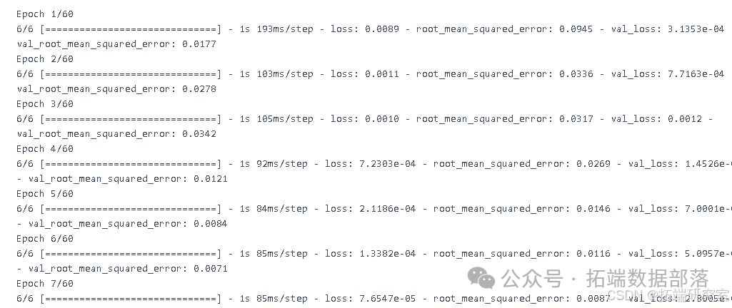

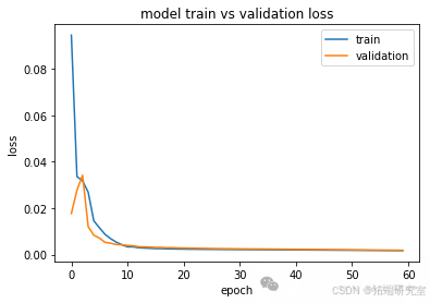
Printing the Model’s Predictions

Through<span>for ind, i in enumerate(lstm.predict(X_test)):</span> this loop structure, predictions are made on the test set<span>X_test</span>, obtaining each prediction result sequentially. This sample-by-sample prediction method helps to evaluate the model’s performance on new data in detail.

<span>printingt, y_tes)</span>This part of the code may be used to print relevant prediction results and true values for comparison and analysis, thus gaining deeper insights into the model’s performance and accuracy.

for ind, i in enumerate(lstm.predict(X_test)):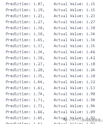

printingt, y_tes)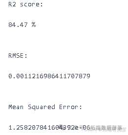

The LSTM model has unique advantages in handling time series data, capable of capturing long-term dependencies.

References[1] Stanford Paper on LSTM Neural Networks for stock prices volatility prediction. http://cs230.stanford.edu/projects_fall_2019/reports/26254244.pdf

The data and code analyzed in this article are shared in themember group. Scan the QR code below to join the group!

Data Acquisition

Reply “Get Data” in the public account backend to obtain free learning materials on data analysis, machine learning, deep learning, etc.

Click “Read the original text” at the end

to obtain the complete code data materials..

This article is excerpted from “Rolling Prediction of SPX Index Financial Time Series Volatility Using LSTM and GARCH”.

Click the title to check past content

R Language GJR-GARCH, GARCH-t, GARCH-ged Analysis of Financial Data Volatility Prediction, Testing, VisualizationR Language GARCH Model Volatility Modeling and Prediction, Backtesting Value at Risk (VaR) Analysis of Stock Market Returns Time SeriesR Language: GARCH Model Stock Trading Volume Research on Dow Jones Stock Market IndexR Language Using Multivariate AR-GARCH Model to Measure Market RiskR Language GARCH Model for Stock Market SP500 Returns Bootstrap, Rolling Estimation Prediction VaR, Fitting Diagnosis and Monte Carlo Simulation VisualizationR Language Univariate and Multivariate (Multivariate) Dynamic Conditional Correlation Coefficient DCC-GARCH Model Analysis of Stock Returns Financial Time Series Data VolatilityR Language Time Series Analysis Models: ARIMA-ARCH / GARCH Model Analysis of Stock PricesGARCH-DCC Model and DCC (MVT) Modeling EstimationR Language Implementation of Futures Volatility Prediction: ARCH vs HAR-RV vs GARCH, ARFIMA Model ComparisonARIMA, GARCH and VAR Model Estimation, Prediction ts and xts Format Time SeriesPYTHON GARCH, Discrete Stochastic Volatility Model DSV Simulation Estimation of Stock Returns Time Series and Monte Carlo VisualizationExtreme Value Theory EVT, POT Exceedance Threshold, GARCH Model Analysis of Stock Index VaR, Conditional CVaR: Diversified Portfolio Risk Measurement AnalysisGARCH Volatility Prediction Regime Switching Trading StrategyFinancial Time Series Models ARIMA and GARCH in Stock Market Prediction ApplicationsTime Series Analysis Models: ARIMA-ARCH / GARCH Model Analysis of Stock PricesR Language Value at Risk: ARIMA, GARCH, Delta-normal Method Rolling Estimation VaR (Value at Risk) and Backtesting Analysis of Stock DataR Language GARCH Modeling Common Software Package Comparison, Fitting Standard & Poor’s SP 500 Index Volatility Time Series and Prediction VisualizationPython Financial Time Series Models ARIMA and GARCH in Stock Market Prediction ApplicationsMATLAB GARCH Model Fitting and Prediction of Stock Market Returns Time Series VolatilityR Language Extreme Value Theory EVT, POT Exceedance Threshold, GARCH Model Analysis of Stock Index VaR, Conditional CVaR: Diversified Portfolio Risk Measurement AnalysisPython Using ARIMA, GARCH Models for Predictive Analysis of Stock Market Returns Time SeriesR Language Time Series Analysis Models: ARIMA-ARCH / GARCH Model Analysis of Stock PricesR Language ARIMA-GARCH Volatility Model Prediction of Stock Market Apple Inc. Daily Returns Time SeriesPython Using GARCH, EGARCH, GJR-GARCH Models and Monte Carlo Simulation for Stock Price PredictionR Language Time Series GARCH Model Analysis of Stock Market VolatilityR Language ARMA-EGARCH Model, Ensemble Prediction Algorithm for SPX Actual Volatility PredictionMATLAB Implementation of MCMC Markov Switching ARMA – GARCH Model EstimationPython Using GARCH, EGARCH, GJR-GARCH Models and Monte Carlo Simulation for Stock Price PredictionUsing R Language for ARIMA + GARCH Trading Strategy on S&P500 Stock IndexR Language Using Multivariate ARMA, GARCH, EWMA, ETS, Stochastic Volatility SV Models for Financial Time Series Data ModelingR Language Stock Market Index: ARMA-GARCH Model and Logarithmic Return Data Exploratory AnalysisR Language Multivariate Copula GARCH Model Time Series PredictionR Language Using Multivariate AR-GARCH Model to Measure Market RiskR Language Time Series Analysis Models: ARIMA-ARCH / GARCH Model Analysis of Stock PricesR Language Using GARCH Model and Regression Model for Stock Price AnalysisGARCH (1,1), MA and Historical Simulation Method VaR ComparisonMATLAB Estimation of ARMA GARCH Conditional Mean and Variance Models