Understanding Dilated Convolutions

Click on the above “Visual Learning for Beginners”, select to add Star or “Top”

Essential information delivered promptly.

Introduction of Dilated Convolutions

Dilated convolutions, also known as dilated convolutions or atrous convolutions, were initially proposed to address the problem of image segmentation. Common image segmentation algorithms typically use pooling layers and convolutional layers to increase the receptive field while also reducing the resolution of the feature map. The process of downsampling and then upsampling causes a loss of precision, thus there was a need for an operation that could increase the receptive field while maintaining the size of the feature map. This led to the birth of dilated convolutions (slightly modified, referenced from [4]). JiuLing Monkey: Understanding the Receptive Field @ JiuLing Monkeyhttps://zhuanlan.zhihu.com/p/113487374 Of course, if we do not use dilated convolutions, how do we compensate for the information loss caused by downsampling? This leads to another approach, which is the well-known skip connection, which can compensate for information during upsampling. Typical topological networks like FCN and U-Net are shown in the figure below. Personally, I believe that if a problem is thought of from different perspectives, different solutions will emerge.

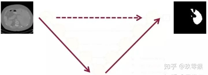
Dilated convolutions were proposed in 2016 at ICLR (International Conference on Learning Representations) and were initially used in the field of image segmentation. They were quickly adopted by DeepMind for applications in speech (WaveNet) and NLP, and they have also played an important role in object detection. Although pixel-wise detection is not required, it is still crucial for the detection of small objects.

2. Principle of Dilated Convolutions

Unlike normal convolutions, dilated convolutions introduce a hyperparameter known as dilation rate, which defines the spacing between the values processed by the convolution kernel. The dilation rate is also referred to as hole size. Here, we use convolution as an example to illustrate the differences between normal convolutions and dilated convolutions, as shown in Figure 2.

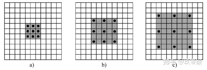
In Figure 2, from left to right are subfigures a, b, and c, which are independently convolved (in contrast to the following Figure 4). The large box represents the input image (the default receptive field is 1), and the black dots represent the convolution kernel, while the gray area indicates the receptive field after convolution (the following calculation formulas are related, and this is a single convolution layer, which can be directly observed).

• a is the normal convolution process (dilation rate = 1), with a receptive field of 3
• b is the dilated convolution with dilation rate = 2, with a receptive field of 5
• c is the dilated convolution with dilation rate = 3, with a receptive field of 8

It can be said that normal convolutions are a special case of dilated convolutions. Additionally, dilated convolutions can increase the receptive field without changing the size of the output feature map (resolution). How can this be understood? To better understand this, we can analyze it from a one-dimensional perspective, which is easier to comprehend.

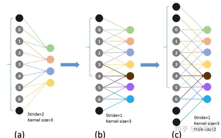
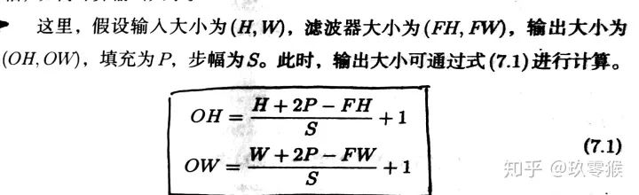
From b and c, it can be seen that whether or not dilated convolutions are used does not affect the size of the output feature map. In other words, the size of the output feature map is independent of the hole size, so dilated convolutions can be used to increase the receptive field while keeping the size of the output feature map unchanged. The factors affecting the size of the output feature map include the size of the input feature map , the size of the convolution kernel , padding , and stride . The calculation formulas are as follows:

Since the feature map size is kept unchanged, this results in a larger computational workload. How can we utilize multi-scale information while keeping the feature map unchanged? Before answering this question, let’s add two points of knowledge: Knowledge Point 1: We know that the larger the value of the neuron’s receptive field, the larger the range of the original image it can touch, which also means it may contain more global and semantically higher-level features; conversely, a smaller value indicates that the features are more local and detail-oriented. Therefore, the value of the receptive field can be used to roughly judge the abstraction level of each layer. Knowledge Point 2: In winning one of the ImageNet competitions, the VGG network’s article stated that its biggest contribution was not the VGG network itself, but a clever observation about stacking convolutions. One 7 x 7 convolution layer is equivalent to stacking three 3 x 3 convolution layers. Such a design can significantly reduce parameters and has a regularization effect; fewer parameters mean less likelihood of overfitting. This is also why most convolution-based deep networks now use small convolution kernels, often using 3 x 3 convolution kernels. Each layer’s convolution kernel is typically of size 3 x 3, and by setting different dilation rates for each layer, the receptive field will vary, thus obtaining multi-scale information. This operation does not affect the size of the feature map, thereby avoiding information loss caused by downsampling while also utilizing multi-scale information, achieving a win-win situation. Obtaining multi-scale information is crucial in visual tasks, especially in dense prediction problems, as it can enhance accuracy, such as in semantic segmentation.

Dense prediction problems such as semantic segmentation … to increase the performance of dense prediction architectures by aggregating multi-scale contextual information (from [1])

3. Calculation of Receptive Field

To make it visually appealing, we will place Figure 2 at the bottom.

From Figure 2, it can be seen that the same convolution can achieve effects similar to and convolutions, all while keeping the number of parameters unchanged (parameters = convolution kernel size + bias). Assuming the size of the dilated convolution kernel is and the hole size is , then the equivalent convolution kernel size is . For example, if the convolution kernel is , then . The formulas are as follows (from [4]):

The calculation formula for the receptive field of the current layer is as follows, where represents the receptive field of the current layer, represents the receptive field of the previous layer, and represents the size of the convolution kernel.

represents the product of the strides of all previous layers (excluding the current layer). The formula is as follows:

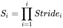
Next, let’s practice with an example. This is Figure 4, which differs from the previous Figure 2. The three images in Figure 2 are independent, while Figure 4 shows continuous convolutions from left to right; they have a top-bottom relationship.

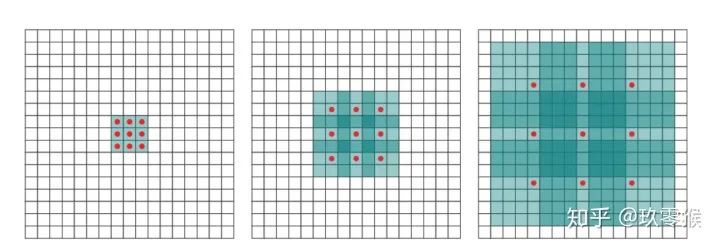
The calculation of the receptive field for the input image: 1 First layer convolution: 3 Second layer convolution:

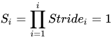
In summary, we get

Third layer convolution:

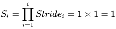
In summary, we obtain

4. Potential Problems and Solutions

Potential Problem 1: The Gridding EffectAssuming we simply stack multiple dilation rate 2 3 x 3 kernels, this issue arises:

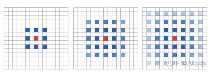
Due to the chessboard-like format of dilated convolutions, the convolution results obtained at a certain layer come from independent collections of the previous layer, which lack interdependence. Therefore, there is no correlation between the convolution results of that layer, leading to a loss of local information. This is fatal for pixel-level dense prediction tasks. Potential Problem 2: Long-ranged information might be not relevant.Information obtained from long distances may lack relevance: the sparse sampling of input signals by dilated convolutions causes a lack of correlation between the information obtained from distant convolutions, affecting classification results. SolutionsFor specific references, see [5,9]

• Panqu Wang, Pengfei Chen, et al**. Understanding Convolution for Semantic Segmentation.//** WACV 2018
• Fisher Yu, et al. Dilated Residual Networks.// CVPR 2017
• Zhengyang Wang, et al.** Smoothed Dilated Convolutions for Improved Dense Prediction.//** KDD 2018.
• Liang-Chieh Chen, et al. Rethinking Atrous Convolution for Semantic Image Segmentation//2017
• Sachin Mehta, et al. ESPNet: Efficient Spatial Pyramid of Dilated Convolutions for Semantic Segmentation.// ECCV 2018
• Tianyi Wu, et al. Tree-structured Kronecker Convolutional Networks for Semantic Segmentation.// AAAI2019
• Hyojin Park, et al. Concentrated-Comprehensive Convolutions for lightweight semantic segmentation.//2018
• Efficient Smoothing of Dilated Convolutions for Image Segmentation.//2019

References1. Yu, Fisher, and Vladlen Koltun. “Multi-scale context aggregation by dilated convolutions.” arXiv preprint arXiv:1511.07122 (2015). (https://arxiv.org/abs/1511.071220)2. Understanding Convolution for Semantic Segmentation (https://arxiv.org/abs/1702.08502)3. Rethinking Atrous Convolution for Semantic Image Segmentation (https://arxiv.org/abs/1706.05587)4. Book “Deep Learning with PyTorch for Object Detection”5. How to Understand Dilated Convolutions (https://www.zhihu.com/question/54149221)6. Analysis of U-Net by the authors of U-Net++ (https://zhuanlan.zhihu.com/p/44958351)7. GIF animation deepening the difference between normal convolutions and dilated convolutions:https://github.com/vdumoulin/conv_arithmetic/blob/master/README.md8. How to Understand Dilated Convolutions9. yyfyan: Summary – Dilated Convolutions (https://zhuanlan.zhihu.com/p/50369448)

Download 1: OpenCV-Contrib Extension Module Chinese Version Tutorial

Reply "Extension Module Chinese Tutorial" in the background of the "Visual Learning for Beginners" public account to download the first Chinese version of the OpenCV extension module tutorial on the internet, covering over twenty chapters including extension module installation, SFM algorithms, stereo vision, target tracking, biological vision, super-resolution processing, etc.

Download 2: Python Visual Practical Project 52 Lectures

Reply "Python Visual Practical Project" in the background of the "Visual Learning for Beginners" public account to download 31 visual practical projects including image segmentation, mask detection, lane detection, vehicle counting, eyeliner addition, license plate recognition, character recognition, emotion detection, text content extraction, facial recognition, etc., to help quickly learn computer vision.

Download 3: OpenCV Practical Project 20 Lectures

Reply "OpenCV Practical Project 20 Lectures" in the background of the "Visual Learning for Beginners" public account to download 20 practical projects based on OpenCV, achieving advanced learning in OpenCV.

Group Chat

Welcome to join the reader group of the public account to exchange with peers. Currently, there are WeChat groups for SLAM, 3D vision, sensors, autonomous driving, computational photography, detection, segmentation, recognition, medical imaging, GAN, algorithm competitions, etc. (which will gradually be subdivided). Please scan the WeChat ID below to join the group, and note: "Nickname + School/Company + Research Direction", for example: "Zhang San + Shanghai Jiao Tong University + Visual SLAM". Please follow the format for remarks; otherwise, you will not be approved. After successful addition, you will be invited to join the relevant WeChat group according to your research direction. Please do not send advertisements in the group; otherwise, you will be removed from the group. Thank you for your understanding.~