↑ ClickBlue text Follow the Extreme City platform Author丨AI Vision EngineSource丨AI Vision EngineEditor丨Extreme City Platform
Extreme City Guide
This article presents the TinyFormer framework for developing Transformers on resource-constrained devices. By implementing a minimal and efficient Transformer on MCUs, it introduces Transformers into the TinyML scenario. Experimental results on CIFAR-10 show that TinyFormer achieves 96.1% accuracy, with an inference latency of 3.9 seconds when running on STM32F746.>> Join the Extreme City CV technology exchange group to stay at the forefront of computer vision.

Paper link: https://arxiv.org/abs/2311.01759
In various embedded IoT applications, developing deep learning models on microcontroller units (MCUs) has garnered significant attention. However, due to severe hardware resource limitations, efficiently designing and deploying state-of-the-art models (e.g., Transformers) on microcontrollers poses substantial challenges. In this paper, the authors propose TinyFormer, a framework specifically designed for developing and deploying resource-efficient Transformers on MCUs. TinyFormer primarily consists of SuperNAS, SparseNAS, and SparseEngine.
Specifically, SuperNAS aims to find suitable super networks from a vast search space. SparseNAS evaluates the best sparse single-path models, including Transformer architectures, from the identified super networks. Finally, SparseEngine efficiently deploys the searched sparse models onto MCUs. To the authors’ knowledge, SparseEngine is the first deployment framework capable of executing sparse model inference with Transformers on a single MCU.
Evaluation results on the CIFAR-10 dataset indicate that TinyFormer can develop effective Transformers with 96.1% accuracy while adhering to hardware constraints of 1MB storage and 320KB memory. Furthermore, compared to the CMSIS-NN library, TinyFormer achieves significant speed improvements in sparse inference, up to 12.2 times. TinyFormer is expected to bring powerful Transformers into the TinyML scenario and greatly expand the scope of deep learning applications.
1. Introduction
In recent years, smart IoT (AIoT) based on IoT technology has become increasingly popular, with microcontroller units (MCUs) receiving widespread attention across various application scenarios. These low-cost, low-power small devices are widely used in plug-and-play scenarios with extreme resource constraints. These devices are typically deployed at the sensor end, collecting the latest data as soon as it is generated.
As a result, Tiny Machine Learning (TinyML) has emerged as a growing field in computer science, aiming to apply machine learning techniques to MCUs for various applications. Some established TinyML applications, such as keyword recognition, anomaly detection, and wake-up functions, only involve a few simple deep learning algorithms. Some high-end applications, such as wildlife detection and food edibility detection, often require powerful deep learning models. However, most of these scenarios are only available on MCUs, posing new challenges for TinyML.
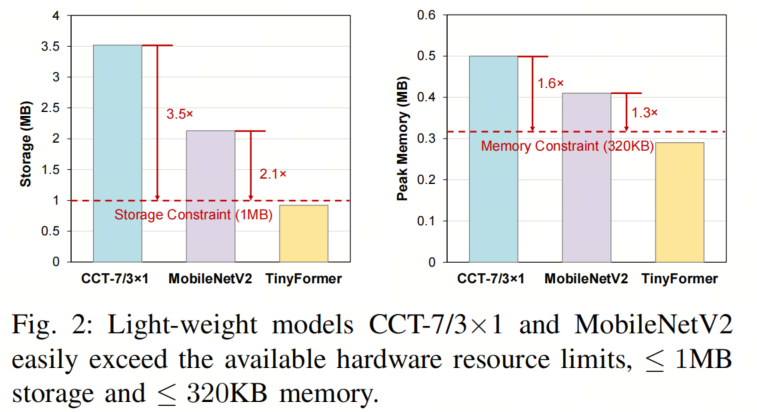
Previously, only relatively simple algorithms or low-end applications could be deployed on such tiny devices. If more powerful deep neural networks could be further deployed on microcontrollers, it would greatly expand the scope of deep learning applications. However, the available resources of MCUs are strictly limited. For example, compared to some edge devices (such as mobile phones and Raspberry Pi), the ARM Cortex-M7 has only 1MB of storage (Flash) and 320KB of memory (SRAM).
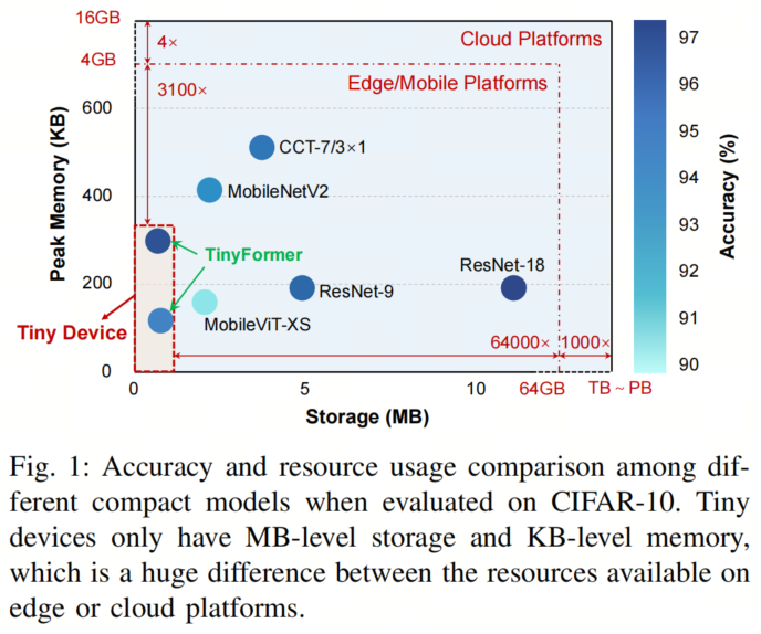
As shown in Figure 1, there is a significant gap between the resources required by deep learning models and the available hardware capacity of microcontrollers. For instance, deploying ResNet-18 with 11 million parameters on a device with 1MB of storage requires reducing at least 90% of the weights, leading to a significant drop in accuracy. Therefore, deploying powerful models on such resource-constrained devices is challenging.
In recent years, Transformer-based models have generally achieved excellent performance in various fields (such as computer vision, speech recognition, and natural language processing). Deploying these powerful Transformer models on MCUs can meet the demands of high-end scenarios in TinyML. However, Transformer models contain a large number of parameters. Compared to mobile devices and cloud platforms, the available memory and storage on MCUs are very limited. Even for lightweight Transformer models that have been developed, it is still difficult to meet their strict resource constraints. Therefore, deploying powerful Transformer models on edge devices or even MCUs remains challenging.
To bring powerful Transformers to MCUs, the authors propose TinyFormer, an effective framework for designing and deploying sparse models on resource-constrained devices. TinyFormer primarily consists of SuperNAS, SparseNAS, and SparseEngine. The goal of SuperNAS is to generate appropriate super networks from a vast search space for further searching. SparseNAS performs model search within the super network and evaluates the hardware constraints and accuracy of the models. Finally, SparseEngine automatically optimizes and deploys the best accuracy model on the target MCU.
The main contributions of this paper are as follows:
- The proposal of the TinyFormer framework for developing Transformers on resource-constrained devices. By implementing a minimal and efficient Transformer on MCUs, it introduces powerful Transformers into the TinyML scenario.
- Through joint search and optimization of sparse configurations and model architectures, TinyFormer generates sparse models with optimal accuracy while meeting hardware constraints.
- The introduction of SparseEngine, the first deployment tool capable of executing sparse model inference with Transformers on external MCUs while ensuring low latency.
Through the synergy of SuperNAS, SparseNAS, and SparseEngine, TinyFormer successfully brings powerful Transformers to resource-constrained devices. Experimental results on CIFAR-10 show that TinyFormer achieves 96.1% accuracy, with an inference latency of 3.9 seconds when running on STM32F746.
Compared to the lightweight Transformer CCT-7/3×1, TinyFormer achieves a 1.04% accuracy improvement while saving 74% of storage space. Thanks to the automated SparseEngine, TinyFormer achieves speed improvements in sparse model inference of up to 12.2× compared to CMSIS-NN.
2. Methodology
A. Overview
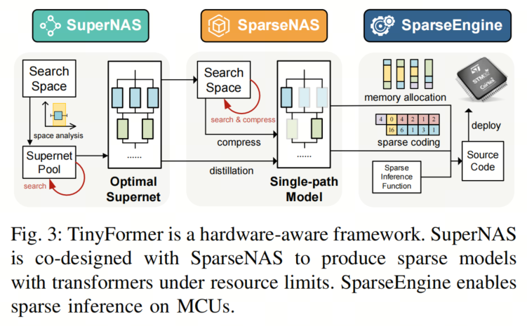
As shown in Figure 3, TinyFormer mainly consists of three parts: SuperNAS, SparseNAS, and SparseEngine. The goal of SuperNAS is to automatically find suitable super networks with Transformer structures in a large search space.
In this work, the super network is constructed as a pre-trained over-parameterized model, from which the following single-path models are sampled. SparseNAS is used to find sparse models with Transformer structures from the super network.
Specifically, sparse pruning is performed in convolutional and linear layers, and full integer quantization (INT8 format) is applied to all layers. During the search phase of SparseNAS, sparse pruning configurations and compression operations are executed simultaneously. Finally, SparseEngine deploys the obtained models to MCUs with sparse configurations, enabling sparse inference to save hardware resources. SparseEngine can automatically generate binary code for STM32 MCUs and supports multiple implementations for efficient sparse inference.
B. SuperNAS: Super Network Architecture Search
When designing the super network structure for searching models to be deployed on MCUs, the authors face a trade-off between model sparsity and capacity. Typically, the accuracy of smaller dense models is limited by capacity, while high sparsity in larger models can lead to a sharp drop in accuracy. The balance between sparsity and capacity should be adjusted according to hardware resource constraints, posing challenges for super network design.
Therefore, the authors propose SuperNAS to automatically design super networks. SuperNAS does not directly output the best single-path model. Instead, it searches for a suitable subset from the search space and constructs a smaller super network. In short, an appropriate super network should meet the following two conditions:
- First, the vast majority of sparse models obtained from the super network should strictly meet resource constraints.
- Second, the average validation accuracy of these models should be as high as possible.
For the design of the super network search space, SuperNAS first analyzes the probability of accepting designs in the search space. Then, SuperNAS randomly samples super network configurations from the search space and evaluates the average accuracy of randomly sampled sparse models in the super network on the validation set. The super network with the best accuracy will be sent to SparseNAS for actual single-path model searching.
1. SuperNAS Search Space:
The search space of SuperNAS includes hyperparameters related to the design of the super network architecture, including the selection of blocks and the number of channels in each selected block. The super network architecture design is shown in Figure 4.
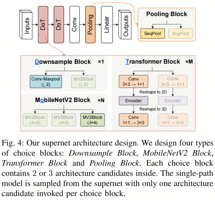
The super network architecture design in TinyFormer is similar to the Single-path One-Shot (SPOS) method. The super network consists of variable selection blocks, and single-path models are sampled at the granularity of selection blocks. The authors construct the super network architecture based on four types of selection blocks: Downsample block, MobileNetV2 block, Transformer block, and Pooling block. Each of the four types of blocks contains multiple different architectural candidates.
In Figure 4, Conv represents standard convolution unless otherwise specified. In the Downsample block, Conv-Maxpool represents standard convolution followed by max pooling. The architecture candidates performing downsampling are marked as . The MobileNetV2 block is an inverted residual block with an expansion factor of . In the Transformer block, Conv represents standard convolution followed by convolution with no padding. Conv is similar to the above expression. The encoder is a standard Transformer encoder, using ReLU as the activation operation to improve computational efficiency on MCUs. SeqPool and AvgPool represent sequence pooling and average pooling, respectively. Single-path models sample from the super network by calling only one architectural candidate per block.
Unlike CNNs, Transformers lack spatial inductive bias and heavily rely on large-scale data for large-scale training. Therefore, the authors insert MobileNetV2 blocks before the Transformer blocks to address this issue. Memory usage is sensitive to the size of the encoder input. To decouple the number of channels from the size of the encoder input, the authors insert 3×3 convolutions and 1×1 convolutions before and after the encoder, referencing MobileViT. This allows the authors to decouple the relationship between channels and encoder input, thereby expanding the search space to explore larger-scale candidate models.
The authors use DoT as the backbone network, which is composed of stacked Downsample blocks, MobileNetV2 blocks, and Transformer blocks. The MobileNetV2 blocks and Transformer blocks in the DoT structure are repeatable, making DoT a more flexible feature extraction architecture. The super network architecture adopts two DoTs as the backbone, followed by some post-processing operations.
2. Search Space Analysis:
The super network search space contains hyperparameters of the super network, such as the number of layers in each selection block, hyperparameters of architectural candidates, etc. The final single-path model is sampled from the super network.
As described in III-B, balancing model sparsity and capacity in search space design is crucial, and the configuration of the search space determines the architecture of the super network and single-path models. Therefore, before sampling the super network, the authors need to evaluate the search space.
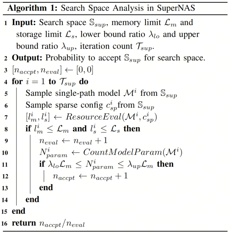
Algorithm 1 shows how the authors analyze the search space. Before the analysis, the authors set hyperparameters and as the lower and upper limits of the single-path model capacity, respectively. The authors randomly sample configurations from the search space and construct sparse single-path models. If the sparse single-path model meets hardware constraints, the authors evaluate the number of parameters, and if the number is within the given boundaries, the authors accept this model.
Finally, the authors calculate statistical probabilities to represent the number of acceptable single-path models in the search space. If the statistical probability exceeds 90%, the authors accept the search space and proceed with further deployment. Otherwise, the authors adjust the search space in advance to avoid unnecessary searches.
3. Super Network Architecture Search:
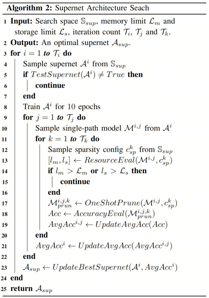
The super network architecture search process is shown in Algorithm 2. For each super network sampled from the search space, the authors perform a simple test before the actual search (TestSupernet in Algorithm 2).
Specifically, the authors randomly sample 100 single-path models from the super network and evaluate the memory usage of each model. If half of the models exceed the memory limit of hardware constraints, the authors skip the search process for that super network.
After the simple test of the super network, the authors take two steps to evaluate its sensitivity to sparsity. First, the authors randomly sample single-path models from the super network. For each single-path model, the authors perform compression using randomly generated sparse configurations to check whether the model occupies more resources. Then, the authors use the average accuracy of these sparse models as the performance metric for the single-path model. Meanwhile, the average metrics of all single-path models are adopted as the final performance metric of the super network. The super network with the highest performance metric will be adopted as the basis for the next stage of searching.
To reduce search costs, the authors evaluate the storage and peak memory usage of sparse models to skip model candidates that do not meet resource requirements. Additionally, the authors adopt a fine-grained one-shot pruning algorithm instead of precise iterative pruning to reduce runtime costs.
C. SparseNAS: Hardware-Aware Sparse Network Search
SparseNAS aims to extract excellent single-path models with sparse configurations and path selection encoding from the super network. Based on path selection encoding, single-path models are extracted from the super network. By performing model compression on sparse configurations and conducting several rounds of fine-tuning, accuracy can be restored to an acceptable level. By repeating the above process, the authors can obtain the model with the highest accuracy.
The single-path model search method is similar to the SPOS method. Unlike the original method, the search step also includes a compression process, such as pruning and quantization. Furthermore, to reduce the costs of training and compression processes, SparseNAS is divided into two stages, known as two-stage NAS.
- In the first stage, SparseNAS aims to find the best sparse single-path model and perform pruning and quantization processes.
- In the second stage, SparseNAS only performs fine-tuning pruning and operations to restore the model’s accuracy.
1. Two-Stage NAS:
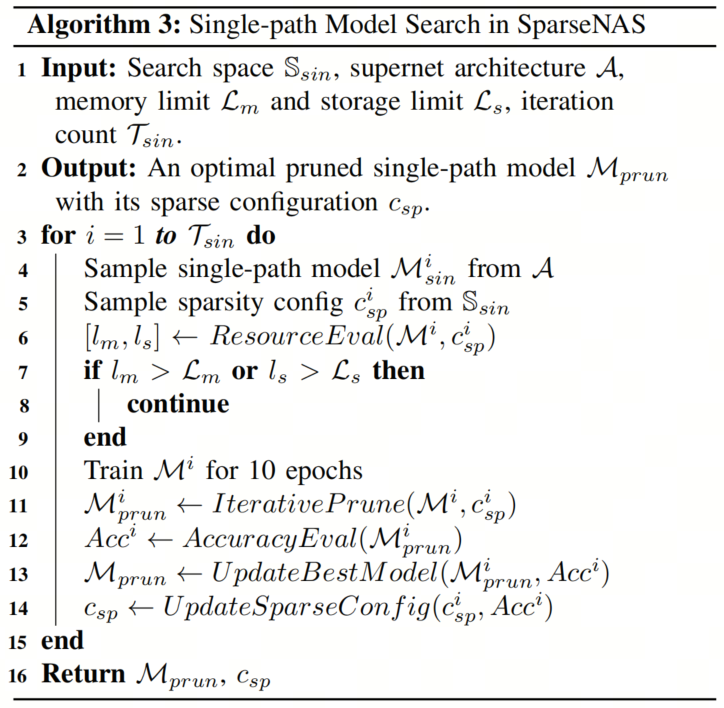
SparseNAS includes the single-path model selection stage and the fine-tuning stage. The first stage of SparseNAS is illustrated in Algorithm 3, which is used for single-path model selection. In the first stage, SparseNAS performs several rounds of training on randomly sampled sparse single-path models, followed by iterative pruning and accuracy evaluation. Only the models with the highest accuracy are selected to enter the second stage for further training. The authors skip model candidates that do not meet hardware constraints by evaluating storage and memory usage.
In the second stage, SparseNAS only performs iterative pruning and fine-tuning on the models selected from the first stage to improve accuracy. After the second stage, the fine-tuned models will be deployed to SparseEngine. The two-stage process can maintain the accuracy of the obtained single-path models while reducing the costs of training and compression.
2. Pruning Method:
Unlike the one-shot pruning method in SuperNAS, SparseNAS adopts the AGP iterative pruning method. The AGP method can avoid significant accuracy drops caused by pruning. The authors only perform pruning on weights in convolutional and linear layers.
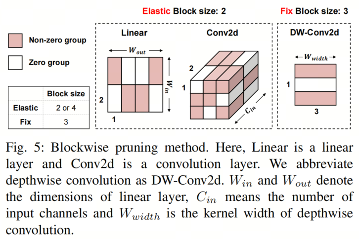
SparseNAS adopts a block pruning method, dividing multiple consecutive weights into a block for pruning. The pruning configuration (sparsity and block size) affects accuracy and hardware resource usage during deployment, and different layers have different sensitivities to pruning configurations. Therefore, the authors adopt a mixed block pruning strategy in convolutional and fully connected layers, as shown in Figure 5. During the mixed block pruning process, SparseNAS selects elastic block sizes (2 or 4) for pruning in each layer. Accordingly, the authors add the pruning configuration for each selected block to the search space. When extracting single-path models, each selected block is set to random sparsity and block size configurations.
As an exception, the block size of deep convolutional layers is fixed at 3. In SparseEngine, the authors apply block convolutions in the width direction to leverage spatial locality of computation. Therefore, the block size of block convolutions is set to 3, with the kernel size fixed at 3×3.
3. Quantization Method:
Compared to floating-point computations on MCUs, integer computations have advantages in latency and power efficiency. Therefore, the authors quantize model weights and activations to INT8 using a post-training quantization (PTQ) algorithm. However, the LayerNorm computation in Transformers cannot be directly quantized. Linear quantization of LayerNorm will lead to significant accuracy drops. The original definition of LayerNorm is as follows:
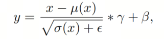
Where and are the mean and variance of the input along the channel direction ( is the number of channels). is the result of the linear transformation before normalization. and are the learnable transformation parameters. is a very small value to prevent division by zero. In linear quantization, the normalized result should be rounded to an integer. However, directly rounding to INT16 will lead to accuracy loss.
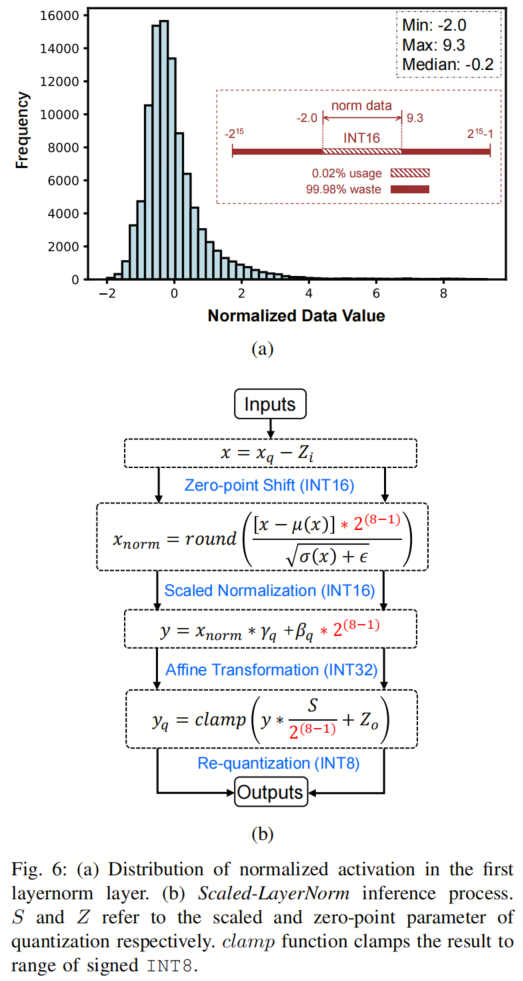
To verify this point, the authors statistically analyze the distribution of LayerNorm in the first DoT architecture. As shown in Figure 6 (a), the normalized data maps to a range of -2.0 to 9.3. Rounding small normalized results in this range to INT16 will lead to significant accuracy loss. On the other hand, the range of INT16 is not fully utilized.
To address this issue, the authors propose Scaled-LayerNorm for integer-only inference instead of LayerNorm. As shown in Figure 6 (b), the authors scale the normalized results by a factor to reduce accuracy loss during the quantization process. The results after linear transformation are stored in INT16 format, along with the scaling factor. In the re-quantization phase, the is folded into the scaling factor S to ensure mathematical equivalence.
By expanding the numerical range of , significant accuracy drops due to large accuracy loss can be avoided. Using this method, the authors achieve a significant speedup in LayerNorm inference while incurring only slight accuracy loss.
D. SparseEngine: Efficient Deployment of Sparse Models
SparseEngine is an automatic deployment tool for deploying sparse transformer models on MCUs. Figure 7 details various aspects of SparseEngine.
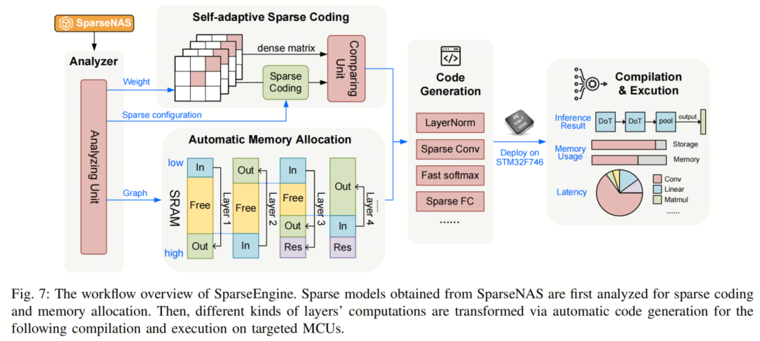
First, the models obtained from SparseNAS are analyzed to extract the required information, including sparse configurations, model architectures, and memory usage. To efficiently utilize the available memory on MCUs, a head-tail alternating allocation strategy is adopted to automatically allocate memory for model inference. Meanwhile, the authors use a block sparse strategy and adopt block run-length encoding (UINT8) for adaptive sparsity.
Specifically, weights are encoded in format, where represents the distance between non-zero blocks as positional information, and represents the th weight in the non-zero block, with a length of . Under the adaptive strategy, weights are stored in sparse format only when the sparse encoding can reduce storage occupancy.
Finally, target code for MCU deployment is generated. Various basic operations for deploying sparse transformer models are implemented, including scaling layer normalization, sparse convolution, and sparse linear layers.
Compared to deployment methods on other MCUs, SparseEngine aims to further exploit sparsity in TinyML deployment and model inference. Sparsity exploitation includes sparse encoding/decoding and sparse computation (convolution and fully connected layers). Additionally, the Softmax operation is optimized for model inference with transformer modules to accelerate inference on MCUs.
1. Sparse Encoding:
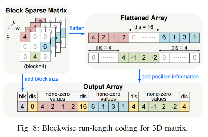
In sparse encoding, the authors adopt 8-bit block run-length encoding for block pruning. The original 3D matrix (tensor) is first flattened into array format. Sparse weights are stored in format, as shown in Figure 8, where dis represents the distance between non-zero blocks as positional information, and represents the th weight in the non-zero block, with a length of . If dis cannot be represented by INT8, the authors insert zero elements.
Compared to Coordinate (COO) and Compressed Sparse Row (CSR) formats, block run-length encoding has a higher compression ratio. The authors only need one element to represent the position of adjacent non-zero weights. The compression ratio of this encoding format can be calculated using the following formula:
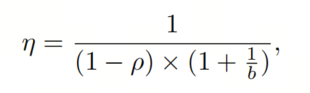
Where represents the compression ratio, represents sparsity, and represents the block size of pruning. Therefore, as sparsity and block size increase, the compression ratio of block run-length encoding can become larger. Combined with the mixed block pruning in SparseNAS, block run-length encoding significantly reduces the required size of sparse encoding.
2. Sparse Convolution:
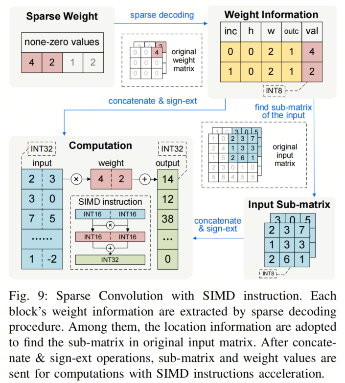
Typically, decoding sparse weights in dense format and performing convolution calculations occupy a large memory footprint. To avoid unnecessary memory usage, the authors perform sparse convolution calculations directly in sparse format. Figure 9 details the sparse convolution calculation. Sparse weights are decoded to obtain coordinates and values. Each weight value corresponds to a submatrix of the input matrix. After extracting the submatrix, the authors perform element-wise matrix multiplication and accumulate the results as output.
Specifically, two weight values are decoded simultaneously, and two corresponding elements are extracted from the submatrix. Then, the two INT8 values are sign-extended to INT16 and concatenated as INT32 format. Thus, the above multiplication-accumulation calculation can be executed using SIMD instructions. Similarly, although the dimensions differ, the sparse linear layer is implemented using the same method.
3. Softmax Optimization:
According to the authors’ analysis, the computation of the Softmax layer is very time-consuming due to the need for exponential operations. The computation of Softmax can be described by the following formula:

Where represents the th value, represents the maximum value (representing the number of elements in a channel). Since the input to Softmax is in INT8 format, the exponential range is from -256 to 0. Therefore, redundant calculations increase with input size. To address this issue, the authors optimize the Softmax operation using a lookup table to reduce redundant calculations.
To compute the negative exponential function, SparseEngine queries the bitmap using the absolute value of the exponential factor as an index. If the corresponding bit exists, SparseEngine retrieves the result from the lookup table and reuses it in the Softmax computation. Otherwise, it computes the exponential function and stores the result in the table, updating the corresponding bit in the bitmap. According to SparseEngine’s evaluation, the memory usage of the bitmap and lookup table typically does not exceed 1.2KB. Since the buffer memory of convolution can be reused during the execution of Softmax optimization, there is no additional memory cost during the computation.
3. Experiments
3.1 Offline Validation
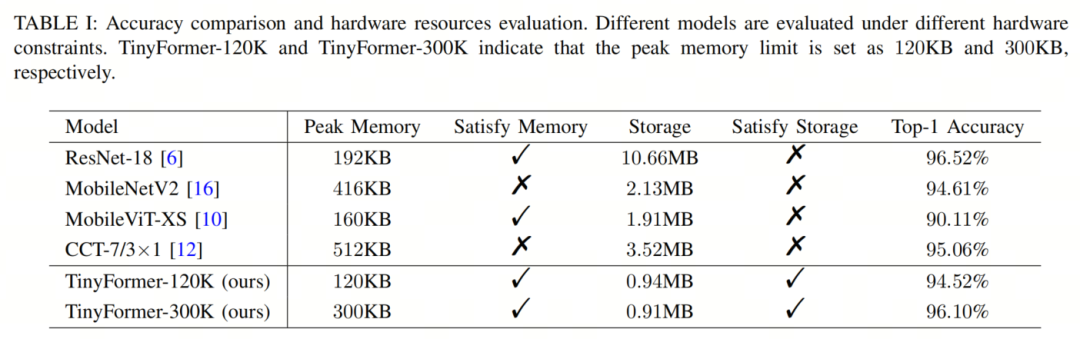
Table I presents the comparison results of the authors’ TinyFormer with other state-of-the-art models. Through the collaborative optimization of SuperNAS and SparseNAS, the authors’ TinyFormer-300K meets hardware constraints and achieves a record accuracy of 96.1% on CIFAR-10. As shown in Figure 4, TinyFormer is designed as a hybrid model, incorporating convolution and Transformer encoder layers.
Compared to other lightweight hybrid models (such as MobileViT-XS and CCT-7/3×1), TinyFormer better combines the advantages of CNNs and Transformers, achieving higher accuracy under limited resources. Compared to CCT-7/3×1 designed for CIFAR-10, TinyFormer-300K improves accuracy while reducing peak memory and storage by 41% and 74%, respectively. Even compared to MobileNetV2 designed for edge device deployment, TinyFormer-300K has advantages in peak memory, storage, and accuracy.
At the same time, TinyFormer-120K is designed for stricter hardware constraints. Compared to MobileViT-XS, TinyFormer-120K improves accuracy by 4.4% with less peak memory and storage. Additionally, TinyFormer-300K shows only a slight decrease in accuracy compared to ResNet-18, while reducing storage usage by 91%.
1. Search Space:
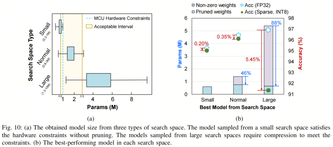
The design of the search space typically affects the size of the sampled models. An inappropriate search space can negatively impact experimental results. As shown in Figure 10 (a), the authors conduct experiments on three different sizes of search spaces, including small, normal, and large. Using hyperparameters and , only the normal search space has an acceptance probability exceeding 90%. The acceptance probabilities of the small and large search spaces are both below 30%. The small search space mainly contains dense models with lower capacity, while the models in the large search space have higher parameter counts and higher sparsity.
Figure 10 (b) shows the performance of the best models obtained from each search space in terms of accuracy and compression ratio. Although the models searched from the small search space do not require pruning, their accuracy is lower than that of other models. The models searched from the large search space have the highest original accuracy. However, they require pruning 88% of the weights to meet hardware constraints, leading to a significant drop in accuracy. On the other hand, the models searched from the normal search space achieve the highest accuracy on MCUs with a good balance between model size and sparsity.
2. Ablation Study:
In this section, the authors present the ablation study of TinyFormer from Table II, including three aspects: whether to use the Transformer module, the number of DoTs, and whether to adopt mixed block size pruning during the search phase. In Table II, TinyFormer refers to the TinyFormer-300K model used in Table I, which includes the Transformer module, two DoTs, and mixed block size pruning.
To understand the impact of the Transformer module in TinyFormer, the authors searched for a CNN model without the Transformer module, labeled as TinyFormer (w/o Tr.). TinyFormer (w/o Tr.) removed the Transformer blocks from the DoT architecture, retaining only the downsample and MobileNetV2 blocks. Compared to TinyFormer (w/o Tr.), TinyFormer achieves better performance with almost the same resource usage, improving accuracy by 1.5%. These results indicate that introducing Transformer-related blocks or layers into TinyML can enhance performance.
Additionally, the authors conducted experiments to evaluate the impact of the number of DoT layers on model accuracy. TinyFormer (Single DoT) originates from a super network containing only a single DoT architecture while meeting the same hardware constraints. In terms of storage, TinyFormer (Single DoT) occupies only 66.8% of the storage limit, resulting in a 1.48% drop in accuracy. When using a single DoT, the main bottleneck for TinyFormer (Single DoT) is memory constraints. In contrast, the model with two DoTs is nearly close to the limits of storage and memory, effectively utilizing resources. Therefore, the authors adopted two DoTs in their basic experiments.
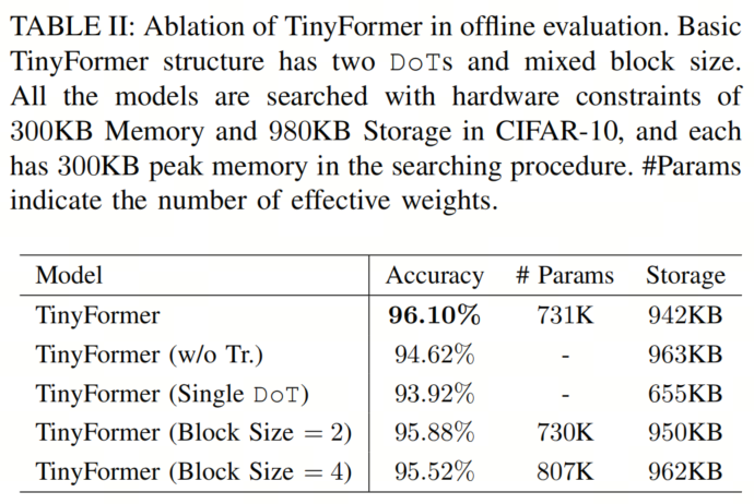
Finally, the authors evaluate the effectiveness of the mixed block size strategy in the SparseNAS stage. Specifically, TinyFormer (Block Size = 2) and TinyFormer (Block Size = 4) represent models with block sizes of 2 and 4 during the block sparsification phase, respectively. Table II shows that larger block sizes can store weights more efficiently within given constraints.
However, setting all patch sizes to 4 can harm model accuracy. Based on these results, the pruning method using mixed block sizes achieves the best balance between block size and effective weight count, resulting in the most suitable model with optimal performance.
3.2. Runtime Evaluation
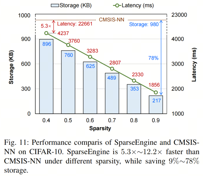
At the runtime level, the authors specifically developed SparseEngine for sparse inference on MCUs. The implementation of SparseEngine successfully reduces the inference time of the highest accuracy search model to 3.8 seconds. To evaluate the performance of SparseEngine, the authors deployed the same sparse model in CMSIS-NN and SparseEngine. As shown in Figure 11, SparseEngine outperforms CMSIS-NN in both inference latency and storage occupancy. By leveraging sparse inference support, SparseEngine significantly reduces storage requirements on MCUs, ranging from 9% to 78%.
Additionally, through dedicated optimizations, SparseEngine achieves speed improvements in inference ranging from 5.3× to 12.2×. Notably, to ensure a fair comparison with CMSIS-NN, the authors needed to ensure that the model fits resource constraints in dense form. Therefore, the models in this experiment could not achieve the highest accuracy.
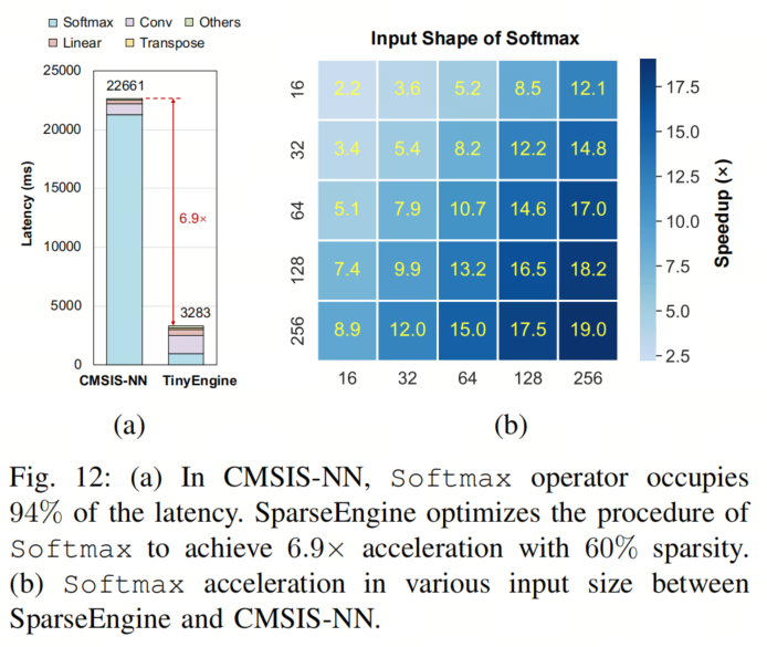
To identify bottlenecks in the inference process, the authors evaluate the runtime breakdown of different layers. As shown in Figure 12 (a), the authors’ findings indicate that the Softmax operation accounts for most of the inference time. Within the Softmax operation, the most time-consuming step is the negative exponential computation. However, the authors find that as the input size increases, the results of the negative exponent can be reused. Leveraging this observation, SparseEngine adopts a bitmap lookup table to reduce redundant calculations and optimize the Softmax operation.
Figure 12 (b) provides a comparison of the inference time of the Softmax operation between CMSIS-NN and SparseEngine, considering different input sizes. Notably, as the input size increases, the optimization effect of SparseEngine becomes more pronounced. In fact, when the input shape is [256×256], SparseEngine achieves a speedup of up to 19× for the Softmax operation.
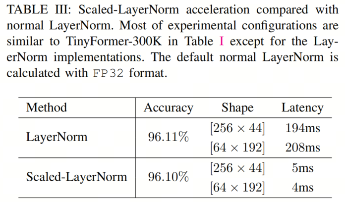
Additionally, the authors conducted an experiment involving the Scaled-LayerNorm in TinyFormer. The authors’ Scaled-LayerNorm uses integer arithmetic computations instead of the previous normal LayerNorm operation, making it more suitable for model inference on MCUs. Furthermore, Scaled-LayerNorm addresses the issue of accuracy loss during quantization by expanding the range of normalized results during the rounding operation. Table III shows the impact of Scaled-LayerNorm on acceleration.
Notably, the accuracy of TinyFormer using Scaled-LayerNorm is nearly the same as that using normal LayerNorm (FP32 format computation), while the inference process is accelerated by 38.8× to 52.0×. These experimental results align with the authors’ expectations, as Scaled-LayerNorm significantly improves the efficiency of LayerNorm inference without a noticeable loss in accuracy. In summary, the experimental results of Softmax and Scaled-LayerNorm validate the authors’ observations and highlight the significant acceleration effects achieved by SparseEngine.
References
[1]. TinyFormer: Efficient Transformer Design and Deployment on Tiny Devices.

Reply “Dataset” in the public account backend to obtain a collection of 100+ resources in various directions of deep learning.
Extreme City Insights
Technical Column: A detailed interpretation column on multimodal large models|Understanding the Transformer series| ICCV2023 paper interpretation| Extreme City LiveExtreme Perspective Dynamics: Welcome to apply for the 2023 Ministry of Education’s Industry-University Cooperation Collaborative Education Project|New Horizons + Smart Brain, “Drones + AI” become good helpers for intelligent road inspection!Technical Review: A 40,000-word detailed explanation of Neural ODE: Using neural networks to characterize non-discrete state changes| What are the details of the transformer? 18 questions about Transformers!

Click to read the original text and enter the CV community
Gain more technical insights