Research on Basic Algorithms and Models of DSP

(Click the public account above for quick follow)

Source: Jiang Shen’s Blog

Link: http://www.techinads.com/archives/41

There is a very excellent DSP company in the United States – M6D (m6d.com). This company is just a startup but has already published 7-8 excellent papers at top conferences like KDD. Recently, I researched their DSP algorithms and would like to share my understanding with everyone, hoping to provide a preliminary understanding of basic algorithms and models in DSP through an example. If there are any inaccuracies in my writing, please feel free to correct me.

This article assumes that everyone has a basic understanding of DSP and the various three-letter acronyms in the RTB ecosystem.

1. Overall Process

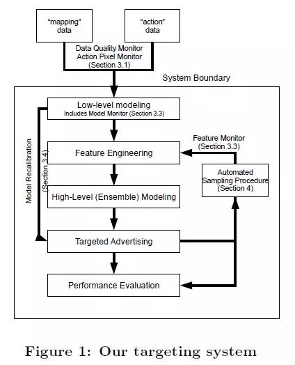
First, let’s take a look at the entire process of M6D’s DSP work:

1. Tracking User Behavior: DSP companies usually embed tracking pixels (i.e., place a 1×1 invisible pixel) on the advertiser’s website. This way, when an internet user visits the advertiser’s website for the first time, they will receive a cookie from the DSP company, allowing the DSP to track this user’s behavior on the advertiser’s website (this data is also called action data). DSP companies also collaborate with third-party websites (e.g., Sina, Tencent) to embed tracking pixels on their sites or purchase user behavior data from DMPs, allowing the tracking of user behavior on these sites (this data is also called mapping data). It is worth mentioning that the cookie recorded by the DSP for a specific user is different from the cookie recorded by third-party websites, DMPs, or exchanges. This requires a process called Cookie Mapping, which is not the focus of this article. For the sake of simplicity, we assume that DSP has completed the Cookie Mapping, and each user has a unique ID identifier.

2. Audience Selection: M6D trains an audience selection model for each campaign (i.e., each advertiser’s promotion activity). This model uses users who have converted on the advertiser’s website (conversion can be defined differently by each advertiser, such as registering as a user, clicking on a specific page, or purchasing a product) as positive examples, and those who have not converted as negative examples (yes, the positive and negative examples are often unbalanced, and sampling and result correction are typically required). After obtaining the model, it estimates the conversion probability p(c | u) for all users, indicating how likely user u is to convert on the advertiser’s website (c represents conversion). Users with a very low conversion probability are filtered out, and target users are divided into different segments based on their conversion probabilities. In this way, we find many target users for each campaign, who are placed in different segments according to their quality.

3. Notify Exchange: The DSP informs the exchange of these target users’ cookies so that when requests with these cookies come in, the exchange will send requests to the DSP’s server.

4. Segment Management: Typically, DSP companies have account managers (operators) who manually set configurations for each campaign. They decide which segments to activate or deactivate based on the industry characteristics and economic conditions of each campaign. For example, for campaigns of small companies with limited budgets, segments with lower conversion probabilities should not be targeted. They also need to set a base price for each segment. Account managers can obtain the average estimated conversion probability for each segment to assist in setting the base price. This step is also where manual influence on placement strategies is most significant.

5. Real-time Bidding: When the exchange sends requests, the DSP receives the following information: current ad placement information, current user’s cookie, and basic information. The DSP needs to decide within 100ms whether to bid for this impression, which campaign’s ad to display, and what the bid amount is (bidding), based on its understanding of the current user and the current ad placement according to its bidding algorithm. If the DSP does not respond within the time limit, the exchange assumes that the DSP has given up on this bidding opportunity.

6. Display Ad: If the DSP wins the opportunity to display, it returns the creative, and the user will see that creative in the ad placement.

7. Track Conversion: Since the DSP has embedded tracking pixels on the advertiser’s website, it can determine whether the user converted after this impression. Based on this data, it calculates conversion rates, average cost per conversion, and compiles reports for the advertiser.

2. Core Algorithms

Steps 2 (Audience Selection) and 5 (Bidding) are the two core steps, where audience selection is an offline computation process, as it can be calculated in advance before the exchange sends requests, while the bidding process needs to be calculated quickly online within 100ms. Below, I will separately introduce the algorithms and models for these two steps, and finally discuss how to evaluate the effectiveness of the algorithms.

Audience Selection:

M6D’s Audience Selection algorithm requires training the following two models for each campaign (the reason for training models independently for each campaign is to protect the privacy of advertisers; data collected from one advertiser’s website cannot be used to optimize another advertiser’s model. For example, data from users who visited the TV purchase page on JD cannot be used to optimize Suning’s model. If JD finds out, they will lose business in the future. Another reason for training models independently for each campaign is that when training data is sufficient, it may yield better results. Of course, privacy concerns are the primary reason):

1. Low-level Model: The purpose of this model is to perform initial selection. All users who have converted on the corresponding advertiser’s website for this campaign are considered positive examples, while others are negative examples (i.e., using action data). The model’s features consist solely of the URLs that users have historically visited (i.e., using mapping data). In other words, the number of possible URLs becomes the dimensionality of the feature space. If a user has visited a specific URL, the corresponding feature value for that URL’s dimension is 1; otherwise, it is 0. It is evident that this leads to an excessively large feature space, so a basic feature selection is performed: removing features that cover fewer than a fixed number of total conversions (e.g., 5) (the threshold can be determined using impression counts, setting it to conversion threshold/average conversion rate). This significantly reduces the number of features. Even after significantly reducing the features, the number is still large, so M6D unsurprisingly uses a linear model for this.

2. High-level Model: The purpose of this model is to perform detailed selection. The sample of this model is the same as that of the Low-level Model, but the features are not limited to the URLs visited by the user; they can include various extracted attribute tags of the user, including interpretable classification tags, unexplainable clustering IDs, topic IDs, and features related to the advertiser’s website. This is where user attribute tags (user profile) play a crucial role. The technology for tagging users is a fundamental skill for many advertising companies, which I won’t elaborate on here. Interestingly, M6D also uses the output of the Low-level Model as one of the features. M6D still chose a linear model for this model, but since the sample size to be predicted is smaller, it can perform some complex calculations. M6D chose a non-linear model (Generalized additive model with smoothing splines) to correct the results.

The reason for dividing into two models is primarily for performance considerations. If all users were predicted using the high-level model, there would be a significant computational burden in feature extraction and prediction. The low-level model, having only URL features, has a simpler feature extraction logic and much lower computational cost. Furthermore, for a campaign’s Low-level Model, the number of non-zero weight features is limited, so it only needs to extract the users corresponding to these non-zero weight URLs to calculate the estimated value (equivalent to a simple retrieval process), without needing to compute estimated values for all users.

Subsequently, each campaign will select target users based on the estimated conversion probabilities p(c|u) predicted by the audience selection model. M6D’s empirical data shows that no more than 1% of users will become target users for a specific campaign. These target users will then be divided into different segments based on different conversion probability thresholds. For example, users with p(c|u) > 0.01 are placed in one segment, and those with 0.01 >= p(c|u) > 0.001 are placed in another segment. The paper does not mention whether a user can be placed in two or more segments, but I believe it should be possible. Each campaign has about 10 to 50 segments. The purpose of segmenting is twofold: first, it facilitates account managers in setting base prices for each segment; second, in the bidding algorithm introduced later, users belonging to the same segment are treated indiscriminately, effectively treating them as belonging to the same class, which alleviates the issue of data sparsity for certain users, which will be explained in detail later.

This is M6D’s audience selection algorithm. It is worth noting that the above steps are offline, meaning they are pre-processed and calculated for each campaign before the exchange’s request arrives. Some places refer to the model that finds more potential users based on a small number of known converting users from the advertiser as a Look-alike Model. I understand that the audience selection model here should also be considered a look-alike model.

Bidding

When the exchange sends requests, the DSP receives the current user’s cookie and some basic user information, as well as the current ad placement information. The DSP needs to find all segments that the user belongs to, which may correspond to multiple campaigns. So which campaign’s ad should be displayed? Here, there is an internal bidding process.

M6D does the following: first, it filters out some unsuitable campaigns based on rules. The main rules include if a user has already seen a certain number of ads from this campaign, then it should not waste advertising costs (this frequency limit is usually called frequency cap). Another main rule is that if a campaign has already reached its daily, weekly, or monthly budget limit, then it will not display ads anymore. For the remaining candidate campaigns, the DSP calculates the most suitable bid for each based on the algorithm and simply selects the highest bid (the bid reflects the current user’s value for that campaign). Careful observers will notice that this is a greedy algorithm, which has room for optimization; we will summarize this at the end.

Next, I will introduce how to calculate the bid for a specific campaign for the current impression opportunity.

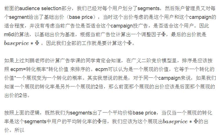
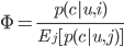
Where u refers to the user, i is the current ad placement (inventory), and c refers to conversion. The denominator calculates the average conversion rate across all ad placements (denoted by j). This denominator is complex to compute, as it requires traversing all ad placements (inventory). However, we know:

Thus, we have:

Therefore, the core part of M6D’s bidding algorithm is to establish two models for each campaign to estimate p(c|u,i) and p(c|u). Considering that the conversion data for each campaign is very limited, training these two models is quite challenging. Therefore, M6D does not differentiate between users within the same segment, allowing the equation to be simplified to:

Where s is the segment. This way, it only needs to train p(c|s,i) and p(c|s). Since the number of segments s is much smaller than the number of users u, the feature space for these two models is significantly reduced, making it easier for the models to yield better results. In fact, M6D also applies a similar trick to i, aggregating similar ad placements together and assigning them the same inventory ID. The goal of this is similar to reducing u to s. M6D’s inventories consist of around 5000, and each campaign has about 10 to 50 segments.

This concludes the modeling process for M6D’s bidding. The remaining task is to train these two models.

p(c|s,i) Model: To obtain the training data for this model, there is a cold start process. Segments must first be exposed to these inventories, marking the impressions that ultimately led to conversion as positive examples and those that did not as negative examples. M6D believes that a conversion is attributed to the last impression seen by the user within the last 7 days. The features for this model consist of two types: segment ID and inventory ID. In other words, each sample has only two non-zero features, one corresponding to the segment ID and the other to the inventory ID. M6D does not combine segment and inventory features, resulting in the assumption that for any segment, the contribution of a specific inventory to the final estimated value is the same. This assumption is reasonable in most cases. Moreover, if these combined features were included in the model, the feature space would significantly increase, which could easily lead to overfitting due to the scarce training data.

p(c|s) Model: This model is essentially the same as the p(c|s,i) model, except that the features only include segment ID.

Both of these models have a very low positive example ratio, so sampling and recalibration are performed. This is a common approach; those unfamiliar can Google the article: “Logistic regression in rare events”.

How much impact does considering inventory have on conversion rate estimation? The following chart illustrates the difference:

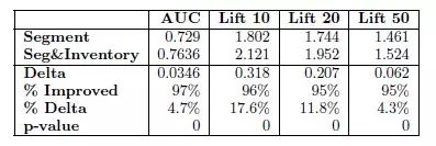
Considering the inventory information, AUC improved by 0.0346, which is quite significant. This Lift is also an evaluation metric, which will be explained in detail later. Here, it can also be seen that the Lift metric has significantly improved.

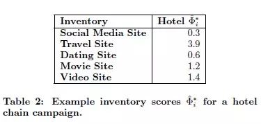
Let’s look at an example. For a hotel advertiser’s campaign, the estimated values for different ad placements vary greatly, with travel-related placements having the highest estimated value and social media the lowest. This indicates that the model has a certain degree of discrimination.

Evaluation

1. Model Evaluation

We typically use AUC to evaluate a model’s ranking ability, but AUC has a problem in that it indiscriminately examines the ranking rationality of all positions in a list. For our audience selection model and conversion rate estimation model, we care more about whether the most reliable examples are ranked at the top. In other words, we pay more attention to the rationality of the ranking of positions in the front of this list. Therefore, M6D uses the Lift metric. The Lift@5% metric measures how much higher the proportion of positive examples is in the top 5% of results compared to the random occurrence rate of positive examples. For a specific definition of Lift, refer to: http://en.wikipedia.org/wiki/Lift_(data_mining)

2. Business Goal Evaluation

For the DSP’s placement effectiveness, M6D mainly looks at two business metrics: one is the conversion rate (PVSVR), which is the number of conversions divided by the number of impressions (i.e., CTR * CVR); the other is CPA, which is the average cost incurred to obtain each conversion.

Most of M6D’s advertisers prefer to purchase impressions on a CPM basis, running ads simultaneously across multiple DSPs, offering the same CPM, and observing who has the highest conversion rate. Therefore, the conversion rate is one of the key metrics for the survival of DSPs.

The conversion rate is independent of price. If a DSP has a 10% lower conversion rate but a 50% lower CPM than others, then advertisers will still choose it because its CPA is lower, meaning that the cost incurred to obtain a conversion is lower.

Thus, the conversion rate of a DSP is tied to profitability. Either improve conversion rates through excellent technology while keeping CPA constant, allowing the DSP to charge higher CPMs to advertisers and earn more money, or sell at lower prices than others, potentially incurring losses. Of course, savvy DSPs will initially invest VC funds at a loss to attract advertisers, as placement can accumulate data, enabling better conversion rates in the future and eventually recouping the costs.

Some advertisers pay per click (CPC), while others have a fixed placement budget, but ultimately, they are all similar, as advertisers will eventually convert this into CPA for comparison (except for those who only care about impression volume).

3. Extended Discussion

The above sections studied M6D’s DSP algorithms and models. I believe there are areas where different approaches could be taken (not necessarily better), and I would like to discuss them with everyone:

1. Conversion rate models in bidding

The previous audience selection model (look-alike model) might have been modeled separately for each campaign because it could achieve better estimation results when training data for each campaign is sufficient. However, the two conversion rate models later on are modeled separately for each campaign primarily due to privacy concerns, as the training data for these two models is too limited. Furthermore, M6D uses conversion as the positive sample, rather than clicks, resulting in even fewer positive examples. Therefore, M6D has to replace u with s for modeling, using the same inventory ID to represent similar ad placements, thereby drastically reducing the feature space, sacrificing bias for lower variance to suppress overfitting and enhance model generalization ability.

If there were not such high privacy requirements, a unified model could be trained using data from all campaigns together. In fact, I have learned that most companies in China do this. Additionally, considering that advertisers in China also care about clicks, a more common modeling approach would be to establish a CTR model (estimated click-through rate = clicks/impressions) p(click|u,i,a), where a refers to a campaign, and a CVR model (conversions/clicks) p(conversion|u,i,a). This way, the training data becomes richer, and predictions can be made directly for each user without needing to estimate for the entire segment. Of course, this result assumes that click and conversion data from one advertiser’s website can positively influence another advertiser’s click and conversion predictions. Under a design of algorithms that does not exhibit obvious bias, it may improve the estimates for most advertisers (especially those with very limited data).

2. Internal bidding mechanism

M6D’s algorithm selects the highest bidding campaign during internal bidding. This is a clear greedy algorithm, and given that each advertiser has budget constraints, it may not be optimal. For example, advertiser A wants users interested in Jordan because they sell Jordan sneakers, but they are a small company that cannot afford to bid too high; advertiser B wants users interested in basketball. At this point, a user who frequently visits the personal page of Jordan on Sina Sports comes along, and after the bidding algorithm, advertiser A bids a maximum of $3, while advertiser B, who has a larger budget, has a base bid of $4, and the bidding algorithm adjusts it to $4.5. In this case, advertiser B’s ad will win the internal bidding. However, there may only be 2-3 impressions available for users interested in Jordan in a day, meaning advertiser A may not fully utilize their daily budget.

This optimization may not be apparent in the early stages of system evolution, but it could become significant as the platform matures and scales up.

3. Considering external competition

M6D’s bidding algorithm is based on value-based bidding without considering competitors’ bids. In other words, the DSP bids based on its perceived value of the impression, regardless of other bids. This could lead to bids that significantly deviate from market prices. For instance, if you believe a shabby old house in the suburbs is worth $2,000 per square meter, but the market price has reached $20,000, you won’t be able to buy the house without adjusting your bid.

Therefore, there is a technique called Bid Landscape Forecasting, which predicts the bidding situation of other competitors. In practical applications, it predicts the relationship between bids and the amount of traffic that can be purchased, essentially creating a curve that shows how much to bid to acquire a certain amount of traffic, allowing for adjustments based on one’s needs. For more details, you can Google the article “Bid Landscape Forecasting in Online Ad Exchange Marketplace”.

A portion of M6D’s algorithm involves account managers setting a base price for segments, and I believe this base price should consider market competition.

4. Traffic prediction and budget control

For advertisers, two main concerns are quality and quantity. Quality means that the ads should be placed in front of those who are likely to be interested in them, while quantity means finding and delivering enough of such ads. Companies like Procter & Gamble are not interested in campaigns that can only cover 1 or 2 people daily, even if those two have a 100% conversion rate.

However, since RTB requires real-time decisions on whether to compete for an impression, DSPs need to anticipate future impressions. For instance, imagine you are on a blind date; you don’t know how many girls will come, but you have the opportunity to date five girlfriends. As each girl meets you sequentially, you must immediately decide whether to go on a date with her. If you have an estimation of the overall quality of the girls or an estimate of how many will come, you can make a more informed choice.

This is also a part of Bid Landscape Forecasting, as it predicts the relationship between bids and the amount of traffic that can be purchased. The available traffic is influenced by both competition and the quality and quantity of that traffic.

5. Click-through rate and conversion rate

M6D directly models conversions rather than separating click-through rates and post-click conversion rates (for some campaigns, clicks on the advertiser’s page are considered conversions; in such cases, there is no difference between the two modeling approaches). Click data is not useful for M6D. If there is a substantial amount of click data, separating modeling may yield better results, as it can utilize click data effectively.

References:

[1] Bid Optimizing and Inventory Scoring in Targeted Online Advertising

[2] Design Principles of Massive, Robust Prediction Systems

[3] Bid Landscape forecasting in Online Ad Exchange Marketplace

[4] Teacher Liu Peng’s “Computational Advertising” course materials: http://www.sheetoo.com/app/course/overview?course_id=200

If you find this article helpful, please share it with more people.

Follow “Algorithm Enthusiasts” to enhance your programming skills.