In signal processing, we often transform signals from the time domain to the frequency domain. Parseval’s theorem tells us that the energy of a signal in the time domain is equal to that in the frequency domain. This article will introduce this theorem and simulate its verification in MATLAB, allowing us to deeply understand this “golden rule” of time-frequency energy conservation.

1. Energy Signals and Power Signals

Before introducing Parseval’s theorem, let’s review the definitions of energy signals and power signals.

The normalized energy of a signal (or simply the energy of the signal) is defined as the energy consumed when the signal voltage (or current) is applied to a unit resistance, denoted as .

If , we call or an energy-bounded signal, abbreviated as an energy signal. In practical applications, general non-periodic signals belong to the category of energy-bounded signals. However, for signals like periodic signals, step functions, and sign functions, it is evident that , which are called energy-unbounded signals. In such cases, we generally do not study the energy of the signal but rather the average power of the signal.

The average power of a signal is defined as the power consumed when the signal voltage (or current) is applied to a unit resistance, denoted as .

If , then we call or a power-bounded signal, abbreviated as a power signal.

Generally speaking, deterministic signals that exist within a finite interval may be energy signals; periodic signals, quasi-periodic signals, and random signals, due to their infinite time duration, are always power signals; not all signals are energy signals or power signals, for example, is neither an energy signal nor a power signal.

2. Parseval’s Theorem

Parseval’s theorem states that the energy of a signal in the time domain is equal to the energy of the signal in the frequency domain, meaning that when a signal undergoes a Fourier transform, its total energy remains unchanged, which complies with the law of energy conservation.

This reflects the distribution of the signal’s energy in the frequency domain, and we call the energy spectral density (abbreviated as energy spectrum). It represents the energy per unit bandwidth, and we usually denote the energy spectrum of as .

Because

, thus the energy of the signal numerically equals the area covered under the curve.

3. MATLAB Simulation Verification

clc;
clear;
close all;
rng default;

fc=1e6;       % Signal frequency
fs=10e6;      % Sampling frequency
N=1000;       % Number of samples
SNR=20 ;      % ADC input signal signal-to-noise (Gaussian) ratio
Ps=1;
Pn=Ps/(10^(SNR/10));
x=sqrt(2*Ps)*cos(2*pi*fc*(0:N-1)/fs)+sqrt(Pn)*randn(1,N);

% Time domain energy calculation
E_time = sum(abs(x).^2);
% Frequency domain energy calculation
X = fft(x);
E_freq = sum(abs(X).^2) / N;

% Display results
fprintf('Time domain energy：%.6f\n', E_time);
fprintf('Frequency domain energy：%.6f\n', E_freq);
fprintf('Energy error (time domain - frequency domain)：%.6e\n', E_time - E_freq);

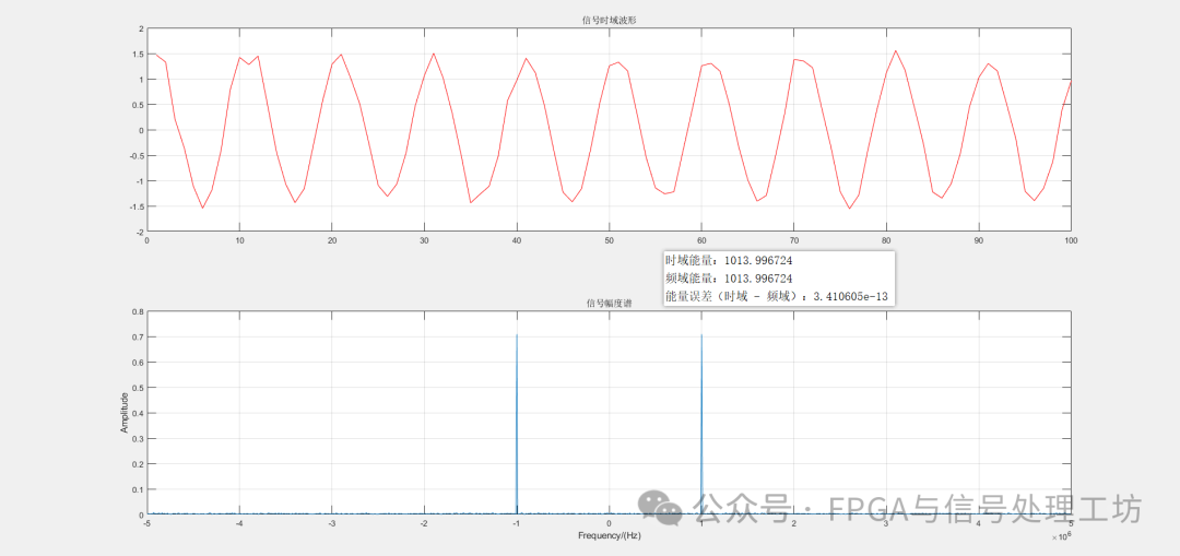
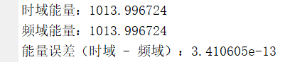
It can be seen that the total energy of a signal in the time domain = its total energy in the frequency domain.

If this article has been helpful to you, please remember to follow our public account, which will continue to update knowledge related to FPGA and signal processing. Thank you!