Like the CPU and memory, the file system and disk I/O are also core functionalities of the Linux operating system.

• The disk provides the most basic persistent storage for the system.

• The file system, built on top of the disk, provides a tree structure for managing files.

File System

1. Inodes and Directory Entries

Everything in Linux is managed by a unified file system, including regular files and directories, as well as block devices, sockets, pipes, etc. The Linux file system allocates two data structures for each file: the inode (index node) and the directory entry (dentry), primarily used to record file metadata and directory structure.

• The inode, abbreviated as inode, is used to record file metadata, such as inode number, file size, access permissions, modification date, and data location. Each inode corresponds to a file, and like the file content, it is persisted to the disk, so inodes also occupy disk space.

• The directory entry, abbreviated as dentry, records the file name, inode pointer, and relationships with other directory entries. Multiple related directory entries form the directory structure of the file system, which is maintained by the kernel as an in-memory data structure, often referred to as the directory entry cache.

In other words, the inode is the unique identifier for each file, while the directory entry maintains the tree structure of the file system. The relationship between directory entries and inodes is many-to-one, or can be understood as multiple aliases for a single file. For example, aliases created for a file through hard links correspond to different directory entries, which essentially link to the same file, hence sharing the same inode.

More specifically, how is file data stored? Is it directly saved to the disk? In fact, the smallest unit of disk read/write is a sector, which is only 512B in size. If every read/write operation were to handle such small units, the efficiency would be very low. Therefore, the file system groups contiguous sectors into logical blocks and manages data using logical blocks as the smallest unit. A common logical block size is 4KB, which consists of 8 contiguous sectors. Below is a diagram illustrating this:

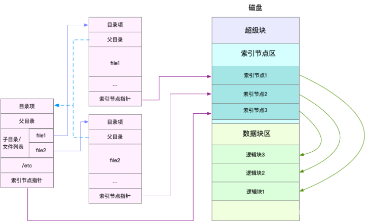
Two points need to be noted here:

First, the directory entry itself is in memory, while the inode is on the disk. As mentioned in the principles of Buffer and Cache, to coordinate the performance differences between slow disks and fast CPUs, file contents are cached in the page cache. Naturally, inodes are also cached in memory to speed up file access.

Second, when the disk is formatted for the file system, it is divided into three storage areas: the superblock, the inode area, and the data block area. The superblock stores the entire file system state; the inode area stores inodes; and the data block area stores file data.

2. Virtual File System

The directory entry, inode, superblock, and logical block constitute the four basic elements of the Linux file system. However, to support various file systems, the Linux kernel introduces an abstraction layer between user processes and file systems, known as the Virtual File System (VFS). VFS defines a set of data structures and standard interfaces supported by all file systems. Thus, user space and other kernel subsystems only need to interact with the unified interface provided by VFS, without concerning themselves with the implementation details of various underlying file systems. The diagram below illustrates the architecture of the Linux file system, which helps to better understand the relationships between system calls, VFS, caches, file systems, and block storage:

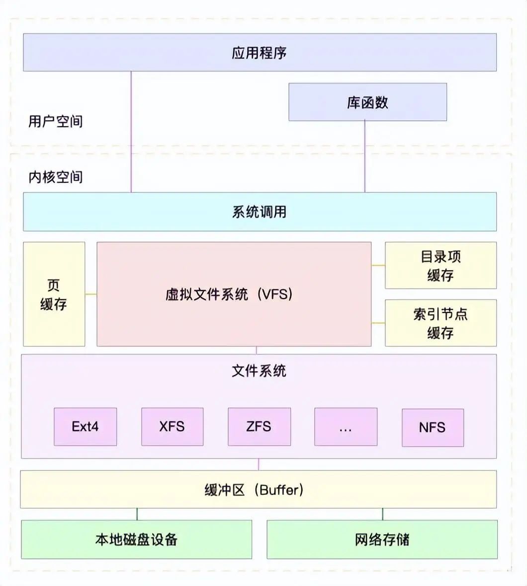
From the diagram, it can be seen that under VFS, Linux can support various file systems, which can be categorized into three types based on storage location:

• Disk-based file systems, which store data directly on the locally mounted disks of the computer, such as EXT4, XFS, OverlayFS, etc.

• Memory-based file systems, which are virtual file systems that do not require any storage space on the disk and only occupy memory, such as the /proc file system and /sys file system (mainly exporting hierarchical kernel objects to user space).

• Network file systems, which are used to access data from other computers, such as NFS, SMB, iSCSI, etc.

These file systems must first be mounted to subdirectories (mount points) in the VFS directory tree before their files can be accessed. For example, during system installation, a root directory (/) must first be mounted, and then other file systems can be mounted under the root directory.

3. File System I/O

Once a file is mounted at a mount point, it can be accessed through it. The standard interface for accessing files provided by VFS is made available to applications via system calls. For example, the cat command sequentially calls open(), read(), and write(). The various differences in file read/write methods also lead to a variety of I/O classifications. Common classifications include buffered vs. unbuffered I/O, direct vs. non-direct I/O, blocking vs. non-blocking I/O, and synchronous vs. asynchronous I/O. Below is a detailed explanation of these four I/O classifications:

The first classification, based on whether standard library caching is utilized, divides file I/O into buffered I/O and unbuffered I/O. Here, “buffered” refers to the cache implemented internally by the standard library. For example, many programs only output data when a newline is encountered; the content before the newline is temporarily cached by the standard library. Thus, buffered I/O refers to using standard library caching to speed up file access, while unbuffered I/O refers to directly accessing files through system calls without using standard library caching. Regardless of whether buffered or unbuffered I/O is used, the final access to files is through system calls. As mentioned earlier, after the system call, page caching is also used to reduce disk I/O operations.

Second, based on whether the operating system’s page cache is utilized, file I/O can be divided into direct I/O and non-direct I/O. To implement direct I/O, the O_DIRECT flag must be specified in the system call; if not specified, the default is non-direct I/O. However, note that direct and non-direct I/O ultimately still interact with the file system. In scenarios such as databases, one may also encounter cases where disk read/write operations bypass the file system, known as raw I/O.

The third classification, based on whether the application blocks its own execution, divides file I/O into blocking I/O and non-blocking I/O. After an application performs an I/O operation, if it does not receive a response and blocks the current thread, it is blocking I/O; if it does not receive a response but does not block the current thread, allowing it to continue executing other tasks, it is non-blocking I/O. For example, when accessing a pipe or network socket, setting the O_NONBLOCK flag indicates non-blocking access; if no settings are made, the default is blocking access.

The fourth classification, based on whether to wait for a response, divides file I/O into synchronous I/O and asynchronous I/O. If an application waits until the entire I/O operation is completed before receiving a response, it is synchronous I/O; if it does not wait for the I/O to complete and continues executing, with the response being notified to the application via event notification once the I/O is complete, it is asynchronous I/O. For instance, when operating on files, if the O_SYNC or O_DSYNC flag is set, it indicates synchronous I/O, where the latter waits for file data to be written to disk before returning, while the former requires that file metadata also be written to disk before returning. Similarly, when accessing a pipe or network socket, setting the O_ASYNC option indicates asynchronous I/O, where the kernel notifies the process via SIGIO or SIGPOLL about the file’s read/write availability.

In summary, whether it is regular files, block devices, network sockets, or pipes, they are all accessed through the unified VFS interface.

4. Observing File System Performance

$ df /dev/sda1
Filesystem 1K-blocks Used Available Use% Mounted on
/dev/sda1 3030824 031670 202712 48 61% /

$ df -h /dev/sda1
Filesystem Size Used Avail Use% Mounted on
/dev/sda1 29G 3.1G 26G 11% /

$ df -i /dev/sda1
Filesystem Inodes IUsed IFree IUse% Mounted on
/dev/sda1 387072 015746 0371260 5% /

By adding the -i parameter, you can check the usage of inodes. The capacity of inodes (i.e., the number of inodes) is set during disk formatting and automatically generated by the formatting tool. When you find that inode space is insufficient but disk space is ample, it is often due to too many small files. Generally, deleting them or moving them to another disk with sufficient inode space can resolve the issue.

Next, how can we check the cache of directory entries and inodes in the file system?

In fact, the kernel uses the Slab mechanism to manage the caches of directory entries and inodes. /proc/meminfo only provides the overall size of Slab; to see the specifics of each Slab cache, you need to check /proc/slabinfo. Running the command below can yield the cache status of all directory entries and various file system inodes:

$ cat /proc/slabinfo | grep -E '^#|dentry|inode'
# name            <active_objs> <num_objs> <objsize> <objperslab> <pagesperslab> : tunables <limit> <batchcount> <sharedfactor> : slabdata <active_slabs> <num_slabs> <sharedavail> 
xfs_inode              0      0    960   17    4 : tunables    0    0    0 : slabdata 000
...
ext4_inode_cache   32104  34590   1088   15    4 : tunables    0    0    0 : slabdata   2306   2306      0hugetlbfs_inode_cache     13     13    624   13    2 : tunables    0    0    0 : slabdata 110
sock_inode_cache    1190   1242    704   23    4 : tunables    0    0    0 : slabdata 54540
shmem_inode_cache   1622   2139    712   23    4 : tunables    0    0    0 : slabdata 93930
proc_inode_cache    3560   4080    680   12    2 : tunables    0    0    0 : slabdata 3403400
inode_cache        25172  25818    608   13    2 : tunables    0    0    0 : slabdata 198619860
dentry             76050 121296    192   21    1 : tunables    0    0    0 : slabdata 577657760

The dentry line indicates the directory entry cache, while the inode_cache line indicates the VFS inode cache; the others represent various file system caches. There are quite a few entries here; you can refer to man slabinfo. In actual performance analysis, slabtop is often used to find the cache type that occupies the most memory:

# Press c to sort by cache size, press a to sort by active object count
$ slabtop
Active/Total Objects (%used): 277970/358914 (77.4%)
Active/Total Slabs (%used): 12414/12414 (100.0%)
Active/Total Caches (%used): 83/135 (61.5%)
Active/Total Size (%used): 57816.88K/73307.70K (78.9%)
Minimum / Average / Maximum Object : 0.01K/0.20K/22.88K

OBJS ACTIVE USE OBJSIZE SLABS OBJ/SLAB CACHESIZE NAME
69804230940%0.19K33242113296Kdentry
16380158540%0.59K12601310080Kinode_cache
58260553970%0.13K1942307768Kkernfs_node_cache
4854130%5.69K9753104Ktask_struct
147213970%2.00K92162944Kkmalloc-2048

From this result, it can be seen that the directory entry and inode occupy the most Slab cache, but it is not large, about 23MB.

Consideration: Does the command find / -name file-name cause an increase in cache, and if so, which type of cache increases?

The find / -name command performs a full disk scan (including memory file systems, disk file systems, etc.), so it will lead to an increase in caches such as xfs_inode, proc_inode_cache, dentry, and inode_cache. Moreover, the next time the find command is executed, it will be much faster because it will mostly look for results directly in the cache. You can compare the outputs of slabtop, free, and vmstat before and after executing the find command for a deeper understanding.

Disk I/O

1. Disk

First, based on the type of storage medium, disks can be divided into two categories: mechanical disks and solid-state disks.

Mechanical disks, also known as hard disk drives (HDD), consist of platters and read/write heads, with data stored in circular tracks on the platters. The smallest read/write unit is a sector, generally 512B in size. When reading or writing data, the head must move to the track where the data is located before accessing it. If the I/O requests are contiguous, there is no need for track addressing, which allows for optimal performance; this is the working principle of sequential I/O. Random I/O requires constant movement of the head to locate data, resulting in slower read/write speeds.

Solid-state disks (SSD) consist of solid-state electronic components, with the smallest read/write unit being a page, typically 4KB or 8KB. Solid-state disks do not require track addressing, and their performance for both sequential and random I/O is significantly better than that of mechanical disks.

Additionally, sequential I/O is always much faster than random I/O for the same disk, for the following reasons:

• For mechanical disks, random I/O requires more head seeking and platter rotation, making it slower than sequential I/O.

• For solid-state disks, although random I/O performance is much better than that of mechanical disks, it still has the limitation of “erase before write.” Random read/write also involves significant garbage collection, so it is still slower than sequential I/O.

• Moreover, sequential I/O can reduce the number of I/O requests through pre-reading, which is another reason for its superior performance.

As mentioned in the previous section, if data were read/written in 512B units each time, the efficiency would be very low. The file system groups contiguous sectors or pages into logical blocks, managing data with logical blocks as the smallest unit. A common logical block is 4KB, which consists of 8 contiguous sectors or one page.

Next, disks can also be classified based on their interfaces, such as IDE, SCSI, SAS, SATA, FC, etc. Different interfaces assign different device names. For example, IDE disks are assigned device names with the prefix hd, while SCSI and SATA disks are assigned names with the prefix sd. If there are multiple disks of the same type, they are numbered in alphabetical order (a, b, c, etc.).

Third, disks can be categorized based on usage architecture. The simplest is to use the disk as an independent disk. Based on needs, the disk can be divided into multiple logical partitions, which are then numbered. For example, the /dev/sda mentioned multiple times can be divided into two partitions: /dev/sda1 and /dev/sda2. Another common architecture is to combine multiple disks into a logical disk, forming a Redundant Array of Independent Disks (RAID) to improve data access performance and enhance data storage reliability.

RAID can be divided into multiple levels based on capacity, performance, and reliability, such as RAID0, RAID1, RAID5, RAID10, etc. RAID0 offers the best read/write performance but does not provide data redundancy, while other RAID levels optimize read/write performance based on data redundancy.

The final architecture combines disks into a network storage cluster, which is then exposed to servers using network storage protocols such as NFS, SMB, iSCSI, etc.

In fact, in Linux, disks are managed as block devices, meaning data is read and written in blocks, supporting random read/write operations. Each block device is assigned a major and minor device number, with the major device number distinguishing device types in the driver, and the minor device number used to number multiple similar devices.

2. Generic Block Layer

To reduce the impact of differences between different block devices, Linux manages various block devices through a unified generic block layer. The generic block layer is an abstraction layer between the file system and disk drivers. It has two functions:

The first function is similar to that of the virtual file system. It provides a standard interface for file systems and applications to access block devices; downward, it abstracts various heterogeneous disk devices into a unified block device and provides a unified framework to manage the drivers of these devices.

The second function is that the generic block layer queues I/O requests from file systems and applications, improving disk read/write efficiency through request queuing and merging.

Sorting I/O requests is also known as I/O scheduling. In fact, the Linux kernel supports four I/O scheduling algorithms: NONE, NOOP, CFQ, and Deadline.

NONE: Strictly speaking, this is not scheduling, as it does not use any scheduler at all and does not process I/O from file systems and applications, commonly used in virtual machines (where disk I/O scheduling is entirely supported by the physical machine).

NOOP: The simplest scheduling algorithm, which is a first-in-first-out queue that only performs basic request merging, commonly used for SSDs.

CFQ: Completely Fair Queuing, the default I/O scheduler for many distributions. It maintains an I/O scheduling queue for each process and evenly distributes each process’s I/O requests over time slices. Similar to CPU scheduling for processes, CFQ scheduling also supports priority scheduling for process I/O, making it suitable for systems running many processes, such as desktop environments and multimedia applications.

Deadline: It creates separate I/O queues for read and write requests, which can improve the throughput of mechanical disks and ensure that requests with deadlines are prioritized. This scheduling algorithm is often used in scenarios with high I/O pressure, such as databases.

3. I/O Stack

Combining the working principles of the file system, disk, and generic block layer, we can view the I/O principles of the Linux storage system as a whole. In fact, we can divide the I/O stack of the Linux storage system into three layers from top to bottom: file system layer, generic block layer, and device layer. See the diagram:

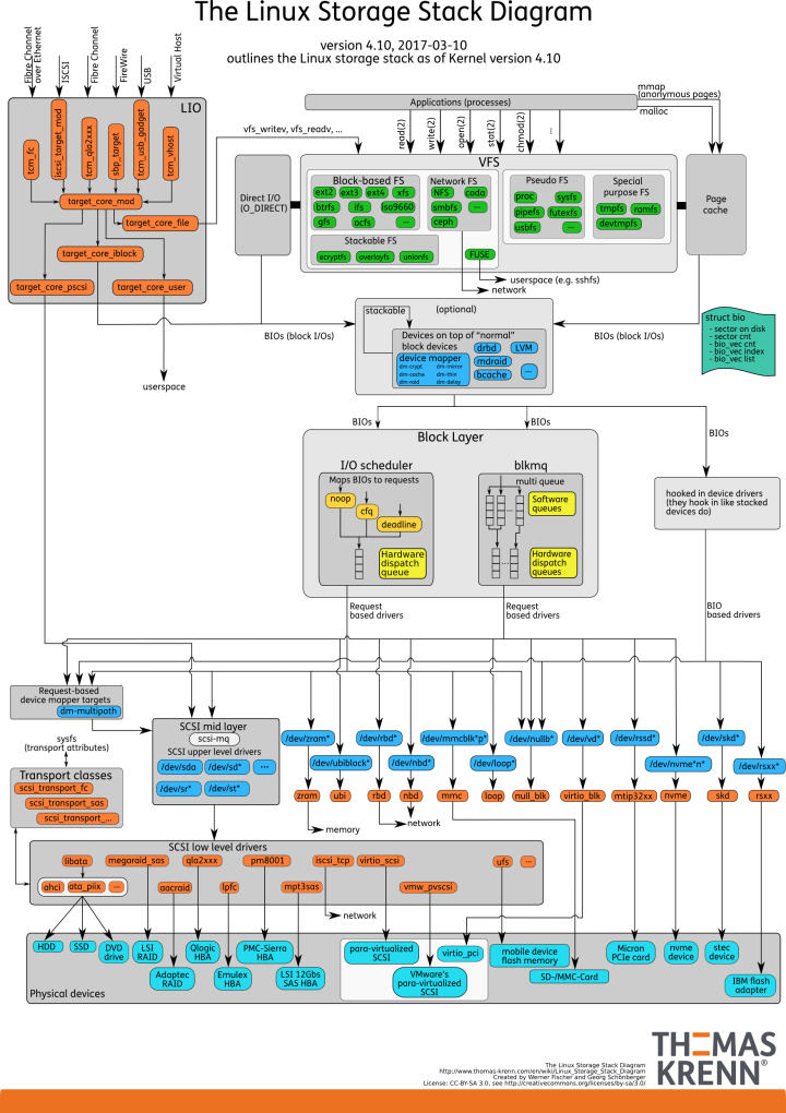
Based on this panoramic view, we can better understand the working principles of the storage system’s I/O:

• The file system layer includes the virtual file system and the specific implementations of various file systems. It first provides standard file access interfaces for upper-layer applications and, downward, stores and manages disk data through the generic block layer.

• The generic block layer is the core of Linux disk I/O, including device I/O queues and I/O schedulers. It queues I/O requests from the file system, reorders and merges them, and then sends them to the lower-level device layer.

• The device layer includes storage devices and their corresponding drivers, responsible for the final physical device I/O operations.

The storage system’s I/O is typically the slowest part of the entire Linux system. Therefore, Linux employs various caching mechanisms to optimize I/O efficiency. For example, to optimize file access performance, it uses page caches, inode caches, directory entry caches, and other caching mechanisms to reduce direct calls to the lower-level block devices. Similarly, to optimize access performance for block devices, it uses buffers to cache data from block devices.

4. Disk Performance Metrics and Observation

Here are five common metrics: utilization, saturation, IOPS, throughput, and response time. These five metrics are the basic indicators for measuring disk performance.

• Utilization refers to the percentage of time the disk is processing I/O. A high utilization (e.g., over 80%) usually indicates a performance bottleneck in disk I/O.

• Saturation indicates the degree of busyness of the disk in processing I/O; a high saturation means there is a serious performance bottleneck. When it reaches 100%, the disk cannot accept new I/O requests.

• IOPS refers to the number of I/O requests per second.

• Throughput refers to the size of I/O requests per second.

• Response time is the time interval from when a request is issued to when a response is received.

Note that utilization only considers whether there is I/O, not the size of I/O; even if it reaches 100%, it may still accept new I/O requests. In scenarios with random read/writes, such as databases and many small files, IOPS better reflects overall system performance. In scenarios with more sequential read/writes, such as multimedia, throughput better reflects overall system performance.

Generally, when selecting disks for application servers, it is essential to conduct benchmark tests on disk I/O performance. The recommended performance testing tool is fio, which tests core metrics such as disk IOPS, throughput, and response time. The metrics obtained from performance tools serve as a basis for subsequent analysis of application performance. Once performance issues arise, these metrics can be used as the limits of disk performance, allowing for an assessment of disk I/O usage.

Next, let’s look at how to observe disk I/O. The recommended tool is iostat, which provides various common performance metrics such as utilization, IOPS, and throughput for each disk; these metrics come from /proc/diskstats. The output interface of iostat is as follows:

# -d -x indicates to display all disk I/O metrics
$iostat -d -x 1
Device r/s w/s rkB/s wkB/s rqm/s wqm/s %rrqm %wrqm r_await w_await aqu-sz rareq-sz wareq-sz svctm %util
loop0 0.00 0.00 0.00 0.00 0.00 0.00 0.00 0.00 0.00 0.00 0.00 0.00 0.00
loop1 0.00 0.00 0.00 0.00 0.00 0.00 0.00 0.00 0.00 0.00 0.00 0.00 0.00
sda 0.00 0.00 0.00 0.00 0.00 0.00 0.00 0.00 0.00 0.00 0.00 0.00 0.00
sdb 0.00 0.00 0.00 0.00 0.00 0.00 0.00 0.00 0.00 0.00 0.00 0.00 0.00

The following diagram explains the specific meanings of these columns:

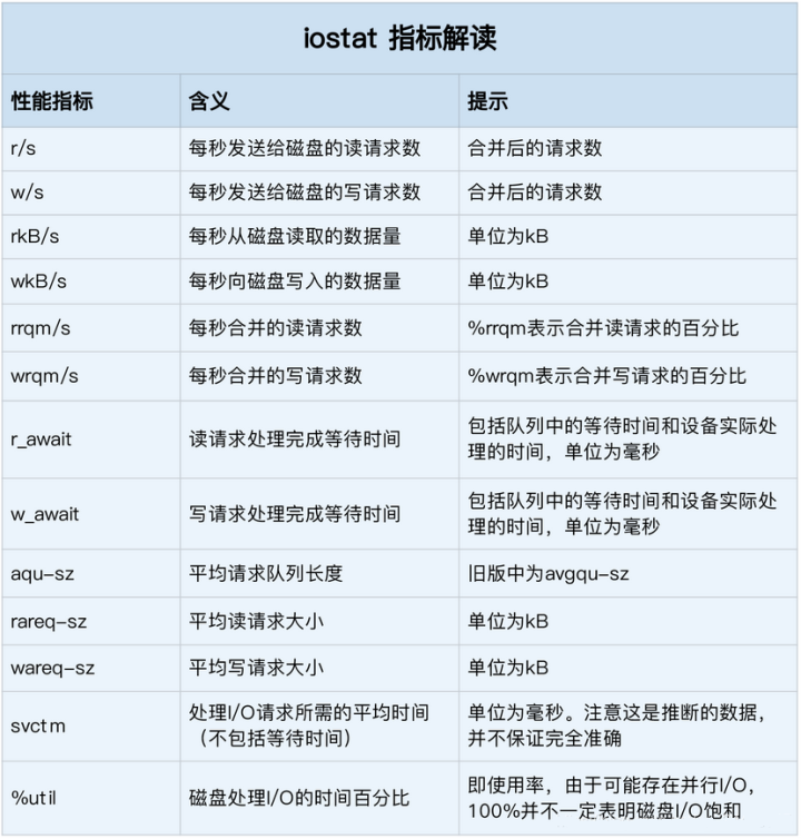
For these metrics, note that %util indicates disk utilization, r/s + w/s indicates IOPS, rkB/s + wkB/s indicates throughput, and r_await + w_await indicates response time. Additionally, while iostat does not directly provide disk saturation, you can compare the observed average request queue length or the waiting time for read/write requests with benchmark test results to comprehensively assess the situation.

Next, let’s look at the I/O situation of each process. iostat can only see the overall I/O performance data of the disk and cannot identify which specific processes are performing disk read/write operations. Two recommended tools for this purpose are pidstat and iotop. The specific usage is omitted here.

-End-