Mathematics contains profound beauty, from fractal geometry to wave equations, from chaotic systems to topological transformations.
1. Fractal Geometry: Dynamic Scaling of the Mandelbrot Set
% Clear workspace and command window
clear all;
clc;

% Set fractal parameters
maxIterations = 100;
resolution = 800;
center = [-0.5, 0];
initialWidth = 3;
zoomFactor = 0.99;

% Initialize figure window
figure('Color', 'black', 'Position', [100, 100, 800, 800]);
axis off;
hold on;

% Create initial grid
x = linspace(center(1)-initialWidth/2, center(1)+initialWidth/2, resolution);
y = linspace(center(2)-initialWidth/2, center(2)+initialWidth/2, resolution);
[X, Y] = meshgrid(x, y);
C = X + 1i*Y;

% Initialize Mandelbrot set calculation
Z = zeros(size(C));
M = zeros(size(C));

% Preallocate color mapping
cmap = jet(maxIterations);
cmap = [000; cmap]; % Add black for non-converging points

% Create video object
video = VideoWriter('mandelbrot_zoom.mp4', 'MPEG-4');
video.FrameRate = 20;
open(video);

% Dynamic scaling loop
for frame = 1:300
    % Calculate Mandelbrot set for current frame
    for k = 1:maxIterations
        Z = Z.^2 + C;
        M(abs(Z) < 2 & M == 0) = k;
    end

    % Draw fractal
    imagesc(x, y, M);
    colormap(cmap);
    axis equal;
    axis off;

    % Add title
    title(sprintf('Mandelbrot Set Zoom - Scale: %.2e', initialWidth), ...
          'Color', 'white', 'FontSize', 14);

    % Capture frame
    F = getframe(gcf);
    writeVideo(video, F);

    % Update zoom parameters
    initialWidth = initialWidth * zoomFactor;
    x = linspace(center(1)-initialWidth/2, center(1)+initialWidth/2, resolution);
y = linspace(center(2)-initialWidth/2, center(2)+initialWidth/2, resolution);
    [X, Y] = meshgrid(x, y);
    C = X + 1i*Y;

    % Reset iteration variables
    Z = zeros(size(C));
    M = zeros(size(C));
end

% Close video
close(video);

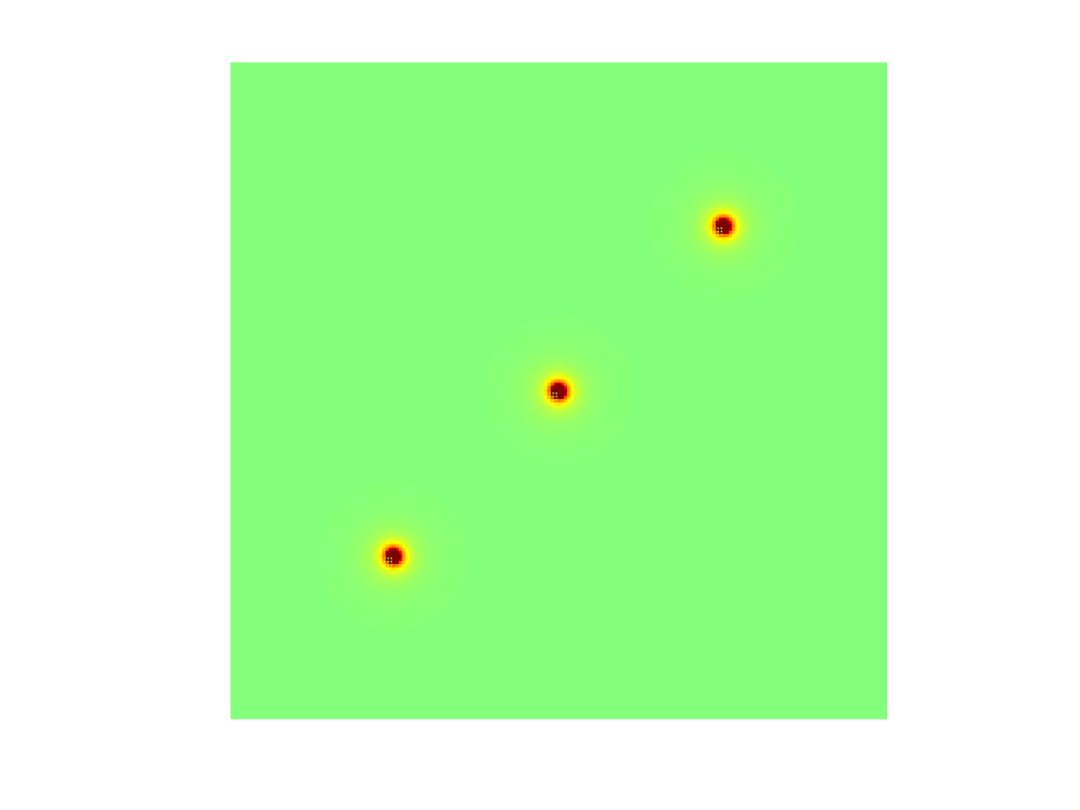
2. Wave Equation: Two-Dimensional Wave Propagation
% Clear workspace and command window
clear all;
clc;

% Set wave equation parameters
N = 200; % Grid size
dt = 0.05; % Time step
dx = 0.1; % Spatial step
c = 1; % Wave speed

% Initialize wave field
u = zeros(N, N);
u_prev = u;

% Add initial disturbances (multiple sources)
sources = [floor(N/2), floor(N/2);
           floor(N/4), floor(N/4);
           floor(3*N/4), floor(3*N/4)];

for i = 1:size(sources, 1)
    u_prev(sources(i,1), sources(i,2)) = 10;
end

% Initialize figure window
figure('Color', 'black', 'Position', [100, 100, 800, 600]);
axis off;
hold on;

% Create video object
video = VideoWriter('wave_propagation.mp4', 'MPEG-4');
video.FrameRate = 20;
open(video);

% Wave simulation
for t = 1:300
    % Update wave field using finite difference method
    for i = 2:N-1
        for j = 2:N-1
            u(i, j) = 2*u_prev(i, j) - u(i, j) + ...
                     (c*dt/dx)^2 * (u_prev(i+1, j) + u_prev(i-1, j) + ...
                     u_prev(i, j+1) + u_prev(i, j-1) - 4*u_prev(i, j));
        end
    end

    % Add boundary conditions (fixed boundaries)
u(1, :) = 0;
u(end, :) = 0;
u(:, 1) = 0;
u(:, end) = 0;

    % Update wave field
    u_prev = u;

    % Visualize wave field
    surf(u, 'EdgeColor', 'none');
    view(0, 90); % Top view
    axis equal;
    axis off;
    colormap(jet);
caxis([-0.5, 0.5]); % Fixed color range
    title(sprintf('2D Wave Propagation - Time: %.2f', t*dt), ...
          'Color', 'white', 'FontSize', 14);

    % Capture frame
    F = getframe(gcf);
    writeVideo(video, F);
end

% Close video
close(video);
3. Chaotic Systems: Evolution of the Lorenz Attractor
% Clear workspace and command window
clear all;
clc;

% Set Lorenz system parameters
sigma = 10;
rho = 28;
beta = 8/3;

% Set initial conditions
x0 = [1, 1, 1];

% Set time parameters
dt = 0.01;
tspan = 0:dt:50;

% Initialize trajectory
x = zeros(length(tspan), 3);
x(1, :) = x0;

% Solve Lorenz system using Euler's method
for i = 2:length(tspan)
    dx = sigma * (x(i-1, 2) - x(i-1, 1));
dy = x(i-1, 1) * (rho - x(i-1, 3)) - x(i-1, 2);
dz = x(i-1, 1) * x(i-1, 2) - beta * x(i-1, 3);

x(i, 1) = x(i-1, 1) + dt * dx;
x(i, 2) = x(i-1, 2) + dt * dy;
x(i, 3) = x(i-1, 3) + dt * dz;
end

% Initialize figure window
figure('Color', 'black', 'Position', [100, 100, 800, 600]);
hold on;
grid on;
set(gca, 'Color', 'black', 'XColor', 'white', 'YColor', 'white', 'ZColor', 'white');

% Create video object
video = VideoWriter('lorenz_attractor.mp4', 'MPEG-4');
video.FrameRate = 30;
open(video);

% Dynamically draw trajectory
trajectory = plot3(x(1,1), x(1,2), x(1,3), 'r', 'LineWidth', 1.5);
current_point = plot3(x(1,1), x(1,2), x(1,3), 'yo', 'MarkerSize', 8, 'MarkerFaceColor', 'y');

xlabel('X');
ylabel('Y');
zlabel('Z');
title('Lorenz Attractor', 'Color', 'white', 'FontSize', 16);
view(45, 45); % Set view angle

% Set axis limits
axis([-20 20 -30 30 0 50]);

% Dynamic drawing
for i = 2:50:length(tspan) % Draw every 50 steps to speed up
    set(trajectory, 'XData', x(1:i,1), 'YData', x(1:i,2), 'ZData', x(1:i,3));
    set(current_point, 'XData', x(i,1), 'YData', x(i,2), 'ZData', x(i,3));

    % Update view angle
    view(45 + 0.1*i, 45);

    % Capture frame
    F = getframe(gcf);
    writeVideo(video, F);
end

% Close video
close(video);
4. Mathematical Analysis: Fourier Series Approximation of Square Wave
% Clear workspace and command window
clear all;
clc;

% Set square wave parameters
T = 2*pi; % Period
N_terms = 50; % Number of Fourier series terms

% Create time vector
t = linspace(0, 3*T, 1000);

% Initialize figure window
figure('Color', 'black', 'Position', [100, 100, 1000, 600]);
hold on;
set(gca, 'Color', 'black', 'XColor', 'white', 'YColor', 'white');
grid on;

% Create video object
video = VideoWriter('fourier_square_wave.mp4', 'MPEG-4');
video.FrameRate = 5;
open(video);

% Draw ideal square wave
square_wave = sign(sin(t));
ideal_plot = plot(t, square_wave, 'r', 'LineWidth', 2);

% Initialize Fourier series
fourier_approx = zeros(size(t));
approx_plot = plot(t, fourier_approx, 'b', 'LineWidth', 2);

% Set axis limits
xlim([0, 3*T]);
ylim([-1.5, 1.5]);
xlabel('Time', 'Color', 'white');
ylabel('Amplitude', 'Color', 'white');
title('Fourier Series Approximation of Square Wave', 'Color', 'white', 'FontSize', 16);
legend('Ideal Square Wave', 'Fourier Approximation', 'TextColor', 'white');

% Dynamically add Fourier terms
for n = 1:2:N_terms*2 % Only consider odd harmonics
    % Calculate current harmonic component
    harmonic = (4/pi) * sin(n*t) / n;

    % Add to Fourier series
    fourier_approx = fourier_approx + harmonic;

    % Update plot
    set(approx_plot, 'YData', fourier_approx);

    % Add current harmonic information
    text(0.5*T, 1.3, sprintf('Added term: (4/π)*sin(%dt)/%d', n, n), ...
         'Color', 'white', 'FontSize', 12);
    text(0.5*T, 1.1, sprintf('Number of terms: %d', (n+1)/2), ...
         'Color', 'white', 'FontSize', 12);

    % Capture frame
    F = getframe(gcf);
    writeVideo(video, F);

    % Pause for observation
    pause(0.2);
end

% Close video
close(video);
Notes:
-
Fractal Geometry: The Mandelbrot set showcases infinite complexity and self-similarity, revealing new details and patterns no matter how much it is magnified.
-
Wave Equation: Two-dimensional wave propagation illustrates the mathematical expression of physical laws and how initial conditions affect the evolution of the system.
-
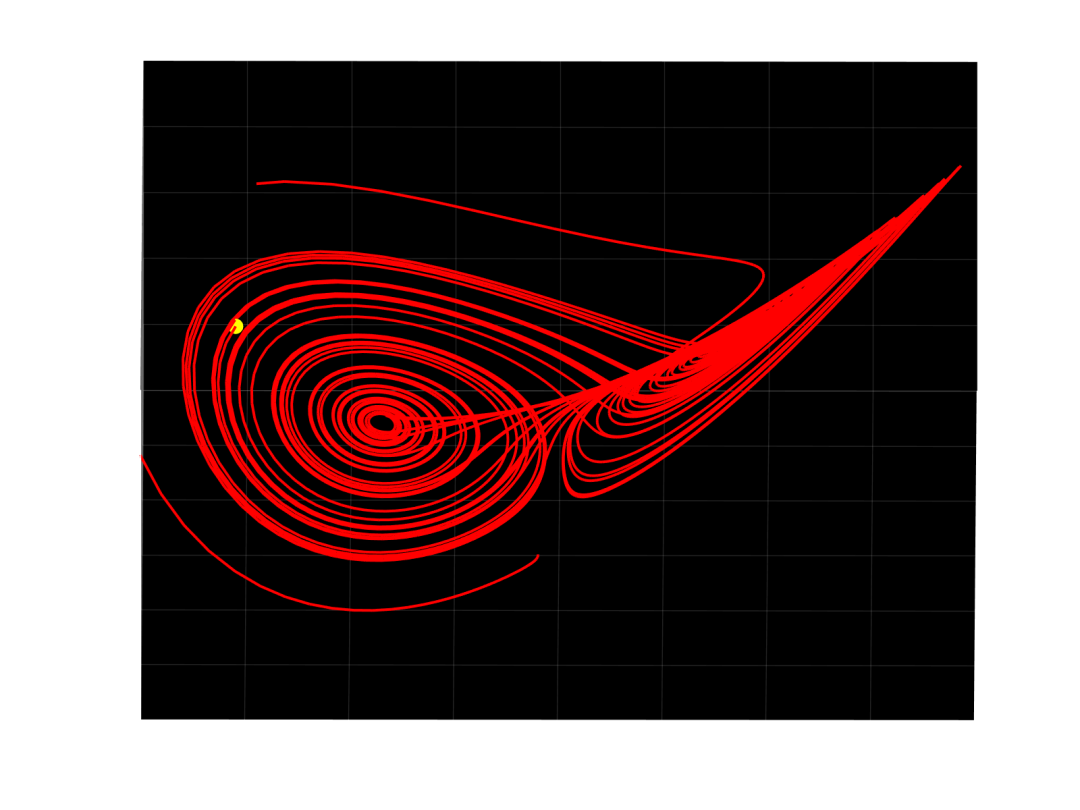
Chaotic Systems: The Lorenz attractor demonstrates unpredictability in deterministic systems and extreme sensitivity to initial conditions.
-
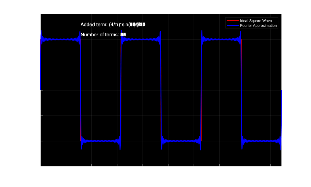
Fourier Analysis: The Fourier series approximation of a square wave shows how complex signals can be approximated using simple sine functions.
These dynamic visualizations not only help us understand mathematical concepts but also showcase the inherent aesthetic value of mathematics. Through MATLAB, we can transform these abstract concepts into intuitive visual experiences, allowing us to appreciate the beauty of mathematics more deeply.
End
 Rotating S to the nth power
Learn more information
Scan to follow the public account
Give a ‘like’ if you find it interesting~