Domenico Marson, Suzana Aulic, Maurizio Fermeglia, Erik Laurini and Sabrina Pricl
Reading time required
minutes
Speed reading only takes 34 minutes
👀
3 Methods
3.1 Box and Simulation Input Parameters Creation
This procedure is used to create a solvated box and the corresponding input files (a topology PRMTOP and an initial coordinates INPCRD files) for the simulation with AMBER. The procedure is valid for creating the input parameter for the single dendrimer or siRNA alone, or the dendrimer-siRNA complex (from now on the name solute is used to indicate any of them in this section) starting from a coordinates PDB file (see Subheadings 3.3-3.5 for the creation of the file for the dendrimer, siRNA and complex, respectively). Open a tleap session with the following command:This procedure is used to create a solvated box and the corresponding input files (a topology PRMTOP and an initial coordinates INPCRD files) for the simulation with AMBER. The procedure is valid for creating the input parameter for the single dendrimer or siRNA alone, or the dendrimer-siRNA complex (from now on the name solute is used to indicate any of them in this section) starting from a coordinates PDB file (see Subheadings 3.3-3.5 for the creation of the file for the dendrimer, siRNA and complex, respectively). Open a tleap session with the following command:
tleap -s
Load the required forcefield library files into AMBER’s tleap software. For parametrizing the dendrimer and the complex load the library and parameters created in Subheading 3.1 together with the general leaprc.gaff library file, while for the siRNA parameterization load the leaprc.RNA.OL3 library file. The last command will load the recommended Amber FF for RNA simulations: the f99 AMBER forcefield with its bsc0 and χOL3 updates . Load also the leaprc.water.tip3p library needed to solvate and add the Na+ and Cl− ions. Finally, load the 3D coordinates files of the solute and save the topology and initial coordinates files for further analysis. All of the above can be obtained by entering the following commands:Load the required forcefield library files into AMBER’s tleap software. For parametrizing the dendrimer and the complex load the library and parameters created in Subheading 3.1 together with the general leaprc.gaff library file, while for the siRNA parameterization load the leaprc.RNA.OL3 library file. The last command will load the recommended Amber FF for RNA simulations: the f99 AMBER forcefield with its bsc0 and χOL3 updates . Load also the leaprc.water.tip3p library needed to solvate and add the Na+ and Cl− ions. Finally, load the 3D coordinates files of the solute and save the topology and initial coordinates files for further analysis. All of the above can be obtained by entering the following commands:
source leaprc.gaff source leaprc.RNA.OL3 source leaprc.water.tip3p loadamberparams dendrimer.frcmod loadamberprep dendrimer.prepi a=loadpdb SOLUTE.pdb saveamberparm a SOLUTE.prmtop SOLUTE.inpcrdNow solvate the solute with TIP3P water molecules (a simple planar three point model for water, commonly used for biological simulations) by creating a cubic solvent box with dimensions ranging at least 1.5 nm from the edges of each solute molecule. In MD simulations is important that the solute does not interact with its images belonging to the adjacent periodic boxes; thus, it is imperative to create a shell of solvent greater than the nonbonded cutoff used during the subsequent MD simulations (0.9 nm, as reported in the parameter cut in Table 1). Accordingly, type the following command:Now solvate the solute with TIP3P water molecules (a simple planar three point model for water, commonly used for biological simulations) by creating a cubic solvent box with dimensions ranging at least 1.5 nm from the edges of each solute molecule. In MD simulations is important that the solute does not interact with its images belonging to the adjacent periodic boxes; thus, it is imperative to create a shell of solvent greater than the nonbonded cutoff used during the subsequent MD simulations (0.9 nm, as reported in the parameter cut in Table 1). Accordingly, type the following command:
solvatebox a TIP3PBOX 15.0Now add the Na+ and Cl−counterions needed to neutralize the solute and to reach a concentration 0.15 M of NaCl, representative of a physiological environment. Two addions commands needed to automatically neutralize the system with the required number of sodium or chlorine ions, as follows:Now add the Na+ and Cl−counterions needed to neutralize the solute and to reach a concentration 0.15 M of NaCl, representative of a physiological environment. Two addions commands needed to automatically neutralize the system with the required number of sodium or chlorine ions, as follows:
addions a Na+ 0 addions a Cl- 0While executing the solvatebox command, tleap will print the total volume (Vol) of the created simulation box, and this information can be used to compute the number of NaCl molecules needed to attain the physiological ionic strength (150 mM) using the following equationWhile executing the solvatebox command, tleap will print the total volume (Vol) of the created simulation box, and this information can be used to compute the number of NaCl molecules needed to attain the physiological ionic strength (150 mM) using the following equation
N u m F o r P h y s C o n c = V o l × 0.15 × 6.022 × 10 − 4 With a third addions command this computed number of sodium and chlorine ions is added to the simulation box. Thus, type:With a third addions command this computed number of sodium and chlorine ions is added to the simulation box. Thus, type:
addions a Na+ NumForPhysConc Cl- NumForPhysConcFinally, save both a topology and an initial coordinates file of the solvated system (required to carry on the subsequent simulations and analysis steps) by typing:Finally, save both a topology and an initial coordinates file of the solvated system (required to carry on the subsequent simulations and analysis steps) by typing:
saveamberparm a SOLUTE.solvated.prmtop SOLUTE.solvated.inpcrd savepdb a SOLUTE.solvated.pdbWith the last command, a reference PDB file containing the model of the solvated simulation box is created.With the last command, a reference PDB file containing the model of the solvated simulation box is created.
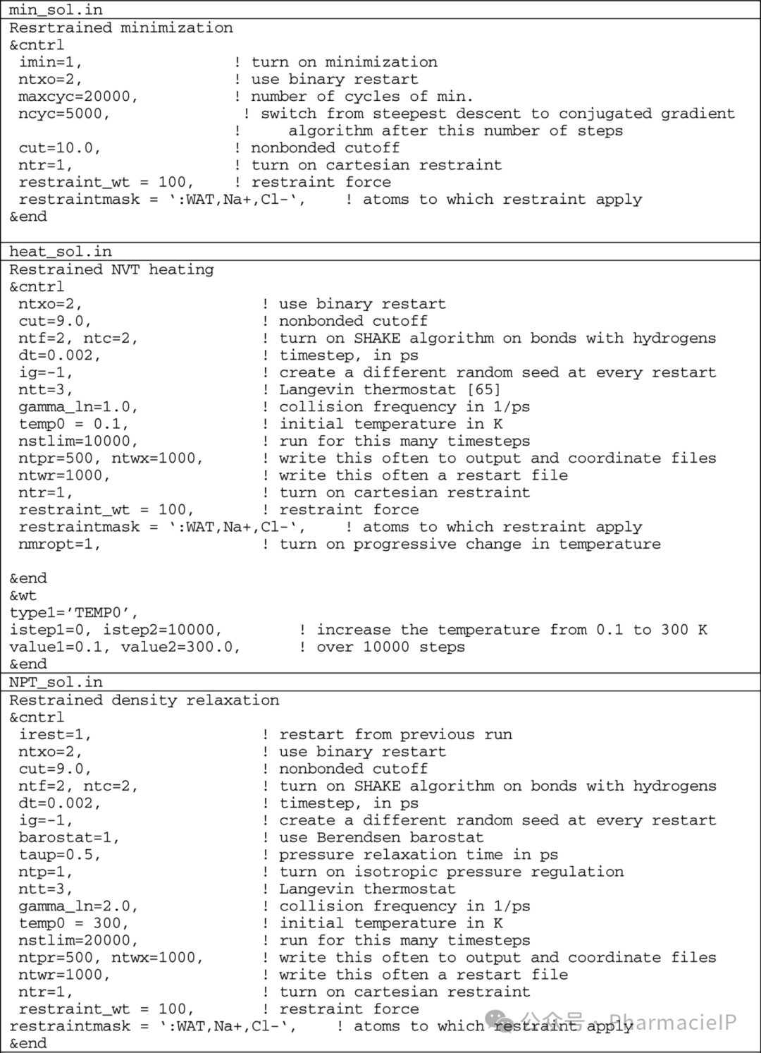
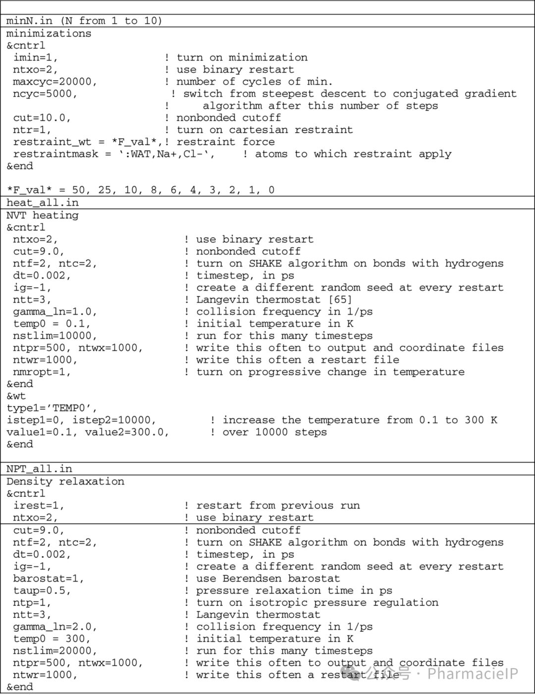
Table 1 List of input files for pmemd. A detailed description of the input parameters can be found in a recent AMBER manual available on line at https://ambermd.org/Manuals.php ( https://ambermd.org/Manuals.php ). The exclamation mark is used to indicate a comment block, as per FORTRAN 90 standard
3.2 Simulation Protocol
This simulation protocol is valid for simulating either the dendrimer or the siRNA molecule alone, or the dendrimer-siRNA complex (i.e., any solute). Throughout all the following MD steps, electrostatic interactions are computed by means of the particle mesh Ewald (PME) algorithm.This simulation protocol is valid for simulating either the dendrimer or the siRNA molecule alone, or the dendrimer-siRNA complex (i.e., any solute). Throughout all the following MD steps, electrostatic interactions are computed by means of the particle mesh Ewald (PME) algorithm.
Before starting any MD simulation, it is fundamental to perform an energy minimization process in order to fix steric clashes and optimize the initial model geometries according to the potential energy function. Also, the solvent box generated according to the protocol reported above needs to be optimized at the desired temperature and pressure conditions. Accordingly, first the solvation box has to be gradually heated to 300 K by performing MD simulations in the NVT ensemble (i.e., under constant number of atoms, volume and temperature conditions) to avoid the creation of air bubbles within the solvent, with positional restraint applied to the solute atoms. Then, while still applying positional restraint to the solute atoms, the system density must be equilibrated at 300 K and 1 atm by means of MD simulations in the NPT ensemble (i.e., under constant number of atoms, pressure and temperature). The solute positional restraints have to be gradually removed in 10 runs of subsequent energy minimizations each performed reducing the force of the positional restraints . Finally, another run of heating in the NVT ensemble followed by density equilibration in the NPT ensemble with the solute free of positional restraint is run (see Table 1) for examples of input files). The following pseudo-code can be used to carry on all of these steps:Before starting any MD simulation, it is fundamental to perform an energy minimization process in order to fix steric clashes and optimize the initial model geometries according to the potential energy function. Also, the solvent box generated according to the protocol reported above needs to be optimized at the desired temperature and pressure conditions. Accordingly, first the solvation box has to be gradually heated to 300 K by performing MD simulations in the NVT ensemble (i.e., under constant number of atoms, volume and temperature conditions) to avoid the creation of air bubbles within the solvent, with positional restraint applied to the solute atoms. Then, while still applying positional restraint to the solute atoms, the system density must be equilibrated at 300 K and 1 atm by means of MD simulations in the NPT ensemble (i.e., under constant number of atoms, pressure and temperature). The solute positional restraints have to be gradually removed in 10 runs of subsequent energy minimizations each performed reducing the force of the positional restraints . Finally, another run of heating in the NVT ensemble followed by density equilibration in the NPT ensemble with the solute free of positional restraint is run (see Table 1) for examples of input files). The following pseudo-code can be used to carry on all of these steps:
   pmemd -O -i min_sol.in -o min_sol.out -r min_sol.rst \
   -p complex.solvated.prmtop -c complex.solvated.inpcrd   pmemd -O -i heat_sol.in -o heat_sol.out -x heat_sol.nc -r heat_sol.rst \
   -p complex.solvated.prmtop -c min_sol.rst -ref min_sol.rst   pmemd -O -i NPT_sol.in -o NPT_sol.out -x NPT_sol.nc -r NPT_sol.rst \
   -p complex.solvated.prmtop -c heat_sol.rst -ref heat_sol.rst   set PREVIOUS=NPT_sol   set N=1 ; while N<=11   pmemd -O -i minN.in -o minN.out -r minN.rst \
   -p complex.solvated.prmtop -c PREVIOUS.rst -ref PREVIOUS.rst   set PREVIOUS=minN   increase N by 1   end   pmemd -O -i heat_all.in -o heat_all.out -x heat_all.nc -r heat_all.rst \
   -p complex.solvated.prmtop -c min10.rst -ref min10.rst   pmemd -O -i NPT_all.in -o NPT_all.out -x NPT_all.nc -r NPT_all.rst \
   -p complex.solvated.prmtop -c heat_all.rst -ref heat_all.rst
In each pmemd command (seeNote1) the option -i and -o specify the input and output (log of some energy and physico-chemical parameters of the simulation) files, option -r specifies the name of the restart file, option -x selects the output coordinates file, option -p selects the solvated complex topology file created by tleap, and options -c and -ref specify the files with the starting and reference coordinates of the system, respectively. In each pmemd command (seeNote1) the option -i and -o specify the input and output (log of some energy and physico-chemical parameters of the simulation) files, option -r specifies the name of the restart file, option -x selects the output coordinates file, option -p selects the solvated complex topology file created by tleap, and options -c and -ref specify the files with the starting and reference coordinates of the system, respectively.
Although a successful energy minimization should get rid of any steric clashes, there are some cases in which the resulting structure is still not perfect (one common example is the presence of intersecting aromatic rings). At least a visual inspection of the final produced configuration is recommended, which can be easily performed loading the produced NPT_all.rst file along with its complex.solvated.prmtop file into a molecular visualization program such as Chimera (https://www.cgl.ucsf.edu/chimera/) or VMD (https://www.ks.uiuc.edu/Research/vmd/ ).Although a successful energy minimization should get rid of any steric clashes, there are some cases in which the resulting structure is still not perfect (one common example is the presence of intersecting aromatic rings). At least a visual inspection of the final produced configuration is recommended, which can be easily performed loading the produced NPT_all.rst file along with its complex.solvated.prmtop file into a molecular visualization program such as Chimera (https://www.cgl.ucsf.edu/chimera/) or VMD (https://www.ks.uiuc.edu/Research/vmd/ ).
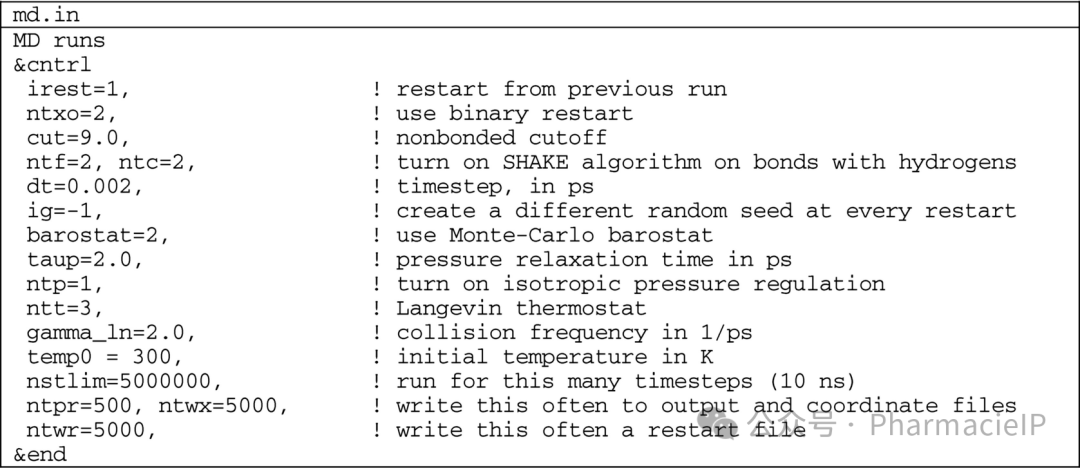
Once optimization of each system is achieved, productive MD simulations can be performed. The required input file is the md.in file reported in Table 1, and 15 subsequent simulations can be carried out with the following pseudo-code command:Once optimization of each system is achieved, productive MD simulations can be performed. The required input file is the md.in file reported in Table 1, and 15 subsequent simulations can be carried out with the following pseudo-code command:
   Set PREVIOUS=NPT_all   set N=1 ; while N<=15   pmemd -O -i md.in -o mdN.out -r mdN.rst \
   -p complex.solvated.prmtop -c PREVIOUS.rst -ref PREVIOUS.rst   set PREVIOUS=mdN   increase N by 1   end
Each of these simulations will run for 10 ns, the first 5 will be discarded as structural equilibration of the solute, and the last 10 produced files (100 ns in total) will be used for subsequent data analysis. Each of these simulations will run for 10 ns, the first 5 will be discarded as structural equilibration of the solute, and the last 10 produced files (100 ns in total) will be used for subsequent data analysis.
3.3 Dendrimer Parametrization
Use any molecular editor software like Avogadro (https://avogadro.cc/) to create a 3D representation of the dendrimer (seeNote2) and save it in PDB format. Use any molecular editor software like Avogadro (https://avogadro.cc/) to create a 3D representation of the dendrimer (seeNote2) and save it in PDB format.
Use AMBER’s antechamber software to assign GAFF atom types to the dendrimer and compute its atomic partial charges via the AM1-BCC method, creating a forcefield library file (PREPIN file) for the dendrimer (seeNote3). This can be achieved with the following command:Use AMBER’s antechamber software to assign GAFF atom types to the dendrimer and compute its atomic partial charges via the AM1-BCC method, creating a forcefield library file (PREPIN file) for the dendrimer (seeNote3). This can be achieved with the following command:
   antechamber -i dendrimer.pdb -fi pdb -o dendrimer.prepi -fo prepi \
   -at gaff -c bcc -nc NET_CHARGE
where the options in order of appearance are: the name of the PDB file, the format, the name of the output file, its format, the forcefield to be applied, the method used to compute the partial charges, and finally the total charge of the dendrimer.where the options in order of appearance are: the name of the PDB file, the format, the name of the output file, its format, the forcefield to be applied, the method used to compute the partial charges, and finally the total charge of the dendrimer.
Use AMBER’s parmchk2 software to create a file (FRCMOD file) for the eventually missing parameters to integrate the dendrimer forcefield library. Execute this command as:Use AMBER’s parmchk2 software to create a file (FRCMOD file) for the eventually missing parameters to integrate the dendrimer forcefield library. Execute this command as:
parmchk2 -i dendrimer.prepi -f prepi -o dendrimer.frcmodwhere the options in order of appearance are: the name of the input PREPI file (created during the execution of the previous antechamber commands), the format of the input file, and the name of the output file. For PAMAM dendrimers , the parameter selected by parmchk2 and reported in the FRCMOD file are accurate enough; however, the user is free to implement any parameter refinement at this stage.where the options in order of appearance are: the name of the input PREPI file (created during the execution of the previous antechamber commands), the format of the input file, and the name of the output file. For PAMAM dendrimers , the parameter selected by parmchk2 and reported in the FRCMOD file are accurate enough; however, the user is free to implement any parameter refinement at this stage.
Follow the steps in Subheadings 3.1 and 3.2 to perform the MD simulation of the dendrimer. The steps in Subheading 3.2 should be repeated three times to obtain the three different trajectories required for further analysis. Follow the steps in Subheadings 3.1 and 3.2 to perform the MD simulation of the dendrimer. The steps in Subheading 3.2 should be repeated three times to obtain the three different trajectories required for further analysis.
3.4 siRNA Model Optimization
Use AMBER’s nab program to create an initial 3D structure of the desired siRNA sequence. This will ensure that the siRNA PDB file created will respect the naming conventions used in the AMBER forcefield. Firstly, create a text file called siRNA.nab with the following code:Use AMBER’s nab program to create an initial 3D structure of the desired siRNA sequence. This will ensure that the siRNA PDB file created will respect the naming conventions used in the AMBER forcefield. Firstly, create a text file called siRNA.nab with the following code:
molecule m; fd_helix( “arna”, “YOUR_RNA_SEQUENCE”, “rna”) putpdb(“siRNA.pdb”, m, “-wwpdb”)Run nab with the following commands to generate the siRNA.pdb file:Run nab with the following commands to generate the siRNA.pdb file:
nab siRNA.nab ./a.outFollow the procedure reported in Subheadings 3.1 and 3.2 to obtain a solvated siRNA structure and an MD equilibrated siRNA trajectory in an aqueous environment. Follow the procedure reported in Subheadings 3.1 and 3.2 to obtain a solvated siRNA structure and an MD equilibrated siRNA trajectory in an aqueous environment.
3.5 Complex Creation and Simulation
Electrostatic interactions are usually at the base of the formation of cationic dendrimer/siRNA complexes, and the intermolecular recognition does not depend on a specific sequence on the nucleic acid fragment (base-aspecific). Nonetheless, any information available from laboratory experiments, literature, or previous knowledge on the particular binding of the specific dendrimer to the given siRNA sequence studied should be taken into consideration when creating the relevant complex model.Electrostatic interactions are usually at the base of the formation of cationic dendrimer/siRNA complexes, and the intermolecular recognition does not depend on a specific sequence on the nucleic acid fragment (base-aspecific). Nonetheless, any information available from laboratory experiments, literature, or previous knowledge on the particular binding of the specific dendrimer to the given siRNA sequence studied should be taken into consideration when creating the relevant complex model.
Using Chimera or VMD extract the final equilibrated structure of the dendrimer from its last data collection trajectory.Using Chimera or VMD extract the final equilibrated structure of the dendrimer from its last data collection trajectory.
With the same software, extract the final equilibrated structure of the siRNA from its last data collection trajectory.With the same software, extract the final equilibrated structure of the siRNA from its last data collection trajectory.
Load both the extracted equilibrated 3D structures of the siRNA and the dendrimer into the visualization software, and place the dendrimer in close proximity of the siRNA yet avoiding visible clashes between their atoms.Load both the extracted equilibrated 3D structures of the siRNA and the dendrimer into the visualization software, and place the dendrimer in close proximity of the siRNA yet avoiding visible clashes between their atoms.
Save the obtained starting 3D structure of the complex to a coordinates PDB file.Save the obtained starting 3D structure of the complex to a coordinates PDB file.
Follow all the steps in Subheadings 3.1 and 3.2 to obtain a solvated complex structure and perform data collection.Follow all the steps in Subheadings 3.1 and 3.2 to obtain a solvated complex structure and perform data collection.
Repeat steps 3–5 two more times, each time rotating the dendrimer and placing it to a different position in relation to the siRNA fragment. At the end of this section, three MD trajectories files will be obtained, each generated from the different dendrimer/siRNA complex starting structures and yet converging to the same equilibrium structure at the end of the corresponding simulation. Should this structural convergence not be achieved, the number of MD simulation must be increased (from 15 to 20 or more) until this condition is satisfied.Repeat steps 3–5 two more times, each time rotating the dendrimer and placing it to a different position in relation to the siRNA fragment. At the end of this section, three MD trajectories files will be obtained, each generated from the different dendrimer/siRNA complex starting structures and yet converging to the same equilibrium structure at the end of the corresponding simulation. Should this structural convergence not be achieved, the number of MD simulation must be increased (from 15 to 20 or more) until this condition is satisfied.
3.6 Dendrimer Analysis
The analysis of every MD simulation should always begin with a careful observation of the relevant trajectories, as some peculiar phenomena taking place during any phase of the calculation can be intuitively identified and, eventually, further investigated. All analysis steps reported here and in the subsequent section have to be repeated for the three replicate trajectories, and the relevant calculated properties or quantities must be reported as average values. As mentioned above for structural model convergence, also the properties of interest obtained from the different MD trajectories must converge to the same value, and if this is not the case, the simulation cannot be trusted. A possible solution for is to run the simulations longer until convergence is achieved. To enter AMBER’s analysis software cpptraj , just type cpptraj on the AMBER command line. Then, execute the following within cpptraj.The analysis of every MD simulation should always begin with a careful observation of the relevant trajectories, as some peculiar phenomena taking place during any phase of the calculation can be intuitively identified and, eventually, further investigated. All analysis steps reported here and in the subsequent section have to be repeated for the three replicate trajectories, and the relevant calculated properties or quantities must be reported as average values. As mentioned above for structural model convergence, also the properties of interest obtained from the different MD trajectories must converge to the same value, and if this is not the case, the simulation cannot be trusted. A possible solution for is to run the simulations longer until convergence is achieved. To enter AMBER’s analysis software cpptraj , just type cpptraj on the AMBER command line. Then, execute the following within cpptraj.
Load the equilibrated 100 ns-long dendrimer MD trajectory by typing:Load the equilibrated 100 ns-long dendrimer MD trajectory by typing:
parm dendrimer.prmtop for i=6;i<16;i++ trajin MD$i.nc 1 last 10 done autoimageUse the command radgyr with the tensor option to compute the dendrimer radius of gyration Rg and the relevant gyration tensor Rg, from which the molecular asphericity b can be obtained (see Subheading 2.2 and Note4):Use the command radgyr with the tensor option to compute the dendrimer radius of gyration Rg and the relevant gyration tensor Rg, from which the molecular asphericity b can be obtained (see Subheading 2.2 and Note4):
radgyr RgyrDendrimer :DENDRIMER_MASK out rgyr_dendrimer_alone.out tensor
Next, use the command radial with the rawrdf and center2 options and selecting the dendrimer as solute to calculate any radial monomer density ρ(r) from the dendrimer center of mass (see Subheading 2.3). Set the maximum radius equal to (Rg × 1.3 + 15) Å, in which Rg is the value of the dendrimer radius of gyration calculated in the preceding step (2). Set spacing = 0.5 Å. This command must be three times, each time selecting i) the water oxygens, ii) the dendrimer terminal nitrogens, and iii) the whole dendrimer atoms, respectively, to obtain corresponding ρ(r) profiles around the center of mass of the dendrimer (seeNote5). Accordingly, type:Next, use the command radial with the rawrdf and center2 options and selecting the dendrimer as solute to calculate any radial monomer density ρ(r) from the dendrimer center of mass (see Subheading 2.3). Set the maximum radius equal to (Rg × 1.3 + 15) Å, in which Rg is the value of the dendrimer radius of gyration calculated in the preceding step (2). Set spacing = 0.5 Å. This command must be three times, each time selecting i) the water oxygens, ii) the dendrimer terminal nitrogens, and iii) the whole dendrimer atoms, respectively, to obtain corresponding ρ(r) profiles around the center of mass of the dendrimer (seeNote5). Accordingly, type:
   radial out radial_density.out 0.5 MAX_RADIUS \
   :WAT@O :DENDRIMER_MASK rawrdf center2   radial out radial_density.out 0.5 MAX_RADIUS \
   :DENDRIMER_MASK@TERMINAL_NITROGEN :DENDRIMER_MASK rawrdf center2   radial out radial_density.out 0.5 MAX_RADIUS \
   :DENDRIMER_MASK :DENDRIMER_MASK rawrdf center2
Now use the command molsurf selecting the dendrimer atoms to compute the relevant accessible surface area (ASA) (see Subheading 2.4). This command has to be issued multiple time, varying the probe option from 0.5 Å to 9.5 Å at 0.3 Å interval. The dendrimer interior cavities and voids can then be identified by plotting the square root of the ASA values thus obtained as a function of the probe radius used (seeNote6). Accordingly, type:Now use the command molsurf selecting the dendrimer atoms to compute the relevant accessible surface area (ASA) (see Subheading 2.4). This command has to be issued multiple time, varying the probe option from 0.5 Å to 9.5 Å at 0.3 Å interval. The dendrimer interior cavities and voids can then be identified by plotting the square root of the ASA values thus obtained as a function of the probe radius used (seeNote6). Accordingly, type:
molsurf ASA_05 :DENDRIMER_MASK out ASA_05.out probe 0.5 molsurf ASA_08 :DENDRIMER_MASK out ASA_08.out probe 0.8 molsurf ASA_11 :DENDRIMER_MASK out ASA_11.out probe 1.1 … molsurf ASA_95 :DENDRIMER_MASK out ASA_95.out probe 9.
3.7 siRNA-Dendrimer Complex Structural Analysis
Load the equilibrated 100 ns-long dendrimer/siRNA complex MD trajectory into AMBER’s cpptraj software by issuing the same commands described in the previous step. Load the equilibrated 100 ns-long dendrimer/siRNA complex MD trajectory into AMBER’s cpptraj software by issuing the same commands described in the previous step.
Within cpptraj, select the dendrimer atoms and use the command radgyr with the tensor option to compute the Rg, Rg and b of the siRNA-bound dendrimer over time. Compare these values with those obtained for the uncomplexed dendrimer in solution obtained at point 2 in Subheading 3.6.Within cpptraj, select the dendrimer atoms and use the command radgyr with the tensor option to compute the Rg, Rg and b of the siRNA-bound dendrimer over time. Compare these values with those obtained for the uncomplexed dendrimer in solution obtained at point 2 in Subheading 3.6.
Next use the command radial with the rawrdf and center2 options and selecting the dendrimer as solute. Follow the same procedure described in step 3 of Subheading 3.6 to set the corresponding values of the maximum radius and spacing. Issue this command 4 times, each time selecting different atoms as solvent (water atoms, the terminal nitrogen atoms, the whole dendrimer atoms and the siRNA atoms, respectively), to obtain the ρ(r) profiles for the selected atoms around the dendrimer center of mass (seeNote5).Next use the command radial with the rawrdf and center2 options and selecting the dendrimer as solute. Follow the same procedure described in step 3 of Subheading 3.6 to set the corresponding values of the maximum radius and spacing. Issue this command 4 times, each time selecting different atoms as solvent (water atoms, the terminal nitrogen atoms, the whole dendrimer atoms and the siRNA atoms, respectively), to obtain the ρ(r) profiles for the selected atoms around the dendrimer center of mass (seeNote5).
3.8 siRNA-Dendrimer Energy of Binding Analysis
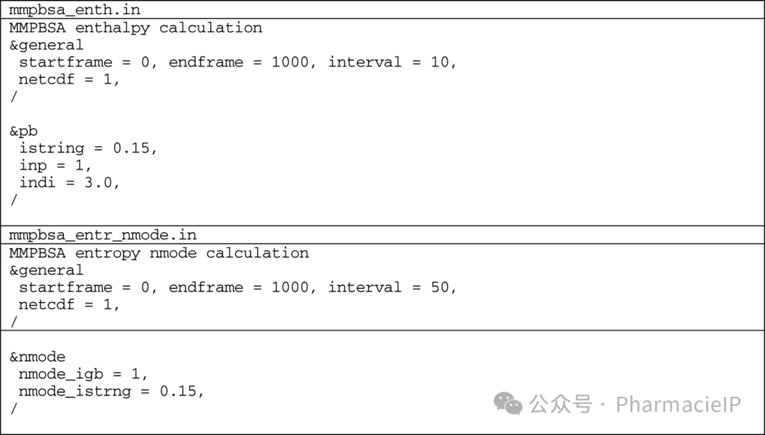
Use AMBER’s MMPBSA.py script to compute the enthalpic contribution to free energy of binding . Select the last two equilibrated MD trajectories obtained for dendrimer, siRNA and their complex, respectively, and pick one every 10 MD frames. The corresponding total number of frames thus will be 200. In the &pb section set inp equal 1 (to separate the dispersion and cavity formation terms) and indi equal 3, as required when dealing with highly charged macromolecules. Also, turn on energy decomposition with &dec, to obtain the contribution of each dendrimer residue to siRNA binding (seeNote 7). Then, move all trajectories and topology files to the same directory, and use the following command line:Use AMBER’s MMPBSA.py script to compute the enthalpic contribution to free energy of binding . Select the last two equilibrated MD trajectories obtained for dendrimer, siRNA and their complex, respectively, and pick one every 10 MD frames. The corresponding total number of frames thus will be 200. In the &pb section set inp equal 1 (to separate the dispersion and cavity formation terms) and indi equal 3, as required when dealing with highly charged macromolecules. Also, turn on energy decomposition with &dec, to obtain the contribution of each dendrimer residue to siRNA binding (seeNote 7). Then, move all trajectories and topology files to the same directory, and use the following command line:
   MMPBSA -O -i mmpbsa_enth.in -o dH_dendrimer_siRNA.out \
   -sp complex.solvated.prmtop -cp complex.prmtop \
   -rp siRNA.prmtop -srp siRNA.solvated.prmtop \
   -lp dendrimer.prmtop -slp dendrimer.solvated.prmtop \
   -y md14.complex.nc md15.complex.nc \
   -yr md14.siRNA.nc md15.siRNA.nc \
   -yl md14.dendrimer.nc md15.dendrimer.nc
where the options -i and -o specify the input and output files, the options -sp, −slp, −srp select the topology files of the solvated complex, dendrimer (ligand) and siRNA (receptor), respectively. Likewise, the options -cp, −lp, −rp and -y, −yl, −yr select the un-solvated topologies for the same systems and their corresponding solvated trajectories, respectively. The content of the mmpbsa_enth.in file is reported in Table 2.where the options -i and -o specify the input and output files, the options -sp, −slp, −srp select the topology files of the solvated complex, dendrimer (ligand) and siRNA (receptor), respectively. Likewise, the options -cp, −lp, −rp and -y, −yl, −yr select the un-solvated topologies for the same systems and their corresponding solvated trajectories, respectively. The content of the mmpbsa_enth.in file is reported in Table 2.
Use AMBER’s MMPBSA.py script to compute the entropic contribution to free energy of binding. Select the same equilibrated trajectories used for enthalpy calculations, and pick one every 50 frames, for a total of 20 analyzed frames. Then, use the following command:Use AMBER’s MMPBSA.py script to compute the entropic contribution to free energy of binding. Select the same equilibrated trajectories used for enthalpy calculations, and pick one every 50 frames, for a total of 20 analyzed frames. Then, use the following command:
   MMPBSA -O -i mmpbsa_entr_nmode.in -o TdS_dendrimer_siRNA.out \
   -sp complex.solvated.prmtop -cp complex.prmtop \
   -rp siRNA.prmtop -srp siRNA.solvated.prmtop \
   -lp dendrimer.prmtop -slp dendrimer.solvated.prmtop \
   -y md14.complex.nc md15.complex.nc \
   -yr md14.siRNA.nc md15.siRNA.nc \
   -yl md14.dendrimer.nc md15.dendrimer.nc
The content of the mmpbsa_entr_nmode.in file is reported in Table 2.The content of the mmpbsa_entr_nmode.in file is reported in Table 2.
As the last step, use the fundamental Gibbs equation, ΔGbind = ΔHbind − TΔSbind, to obtain the corresponding free energy of binding between the dendrimer and the siRNA (see Subheading 2.5, Notes 8 and 9).As the last step, use the fundamental Gibbs equation, ΔGbind = ΔHbind − TΔSbind, to obtain the corresponding free energy of binding between the dendrimer and the siRNA (see Subheading 2.5, Notes 8 and 9).
Table 2 List of input files for energy of binding calculations. A detailed description of the input parameters can be found in a recent AMBER manual available on line at https://ambermd.org/Manuals.php ( https://ambermd.org/Manuals.php )
👀
4 Notes
The commands presented to perform energy minimization and MD simulations use the pmemd software of AMBER in its serial implementation, e.g., running on a single core. Given that powerful computational resources are commonly available to date, the single-core protocol was proposed in order to adopt a platform-agnostic approach. However, AMBER offers a parallel version of the software, pmemd.MPI, and also a GPU-based version called pmemd.cuda. Without entering in the technical details of the precision of the GPU-based code, our suggestion is to use it for every step of MD simulations whenever an appropriate hardware is available. To perform the energy minimization, however, the parallel pmemd.MPI version is always recommended.
为了执行能量最小化和分子动力学模拟,所提供的命令使用 AMBER 的pmemd软件的串行版本,例如在单核心上运行。由于现今计算资源相对充足,选择串行协议旨在采用平台无关的方式。然而,AMBER 还提供了并行版本 pmemd.MPI,以及 GPU 版本 pmemd.cuda。尽管 GPU 版本的代码精度未在此深入讨论,但我们建议在有合适硬件的情况下,尽可能使用 GPU 版本来执行每一步的分子动力学模拟。然而,在进行能量最小化时,仍然推荐使用并行的 pmemd.MPI 版本。
The regularly self-similar nature of dendrimers usually leads to a straightforward subdivision of their structure in a small number of repetitive moieties. Generally, for any dendrimer a central core unit, a repeating entity, and a terminal group can be identified, as shown in Fig. 1. Moreover, to build different dendrimer generations (G), successive layers of the repeating units can be simply added (Fig. 1). This dendrimer model building is also very practical as it allows for the fast FF parameterization of each individual dendrimer fragment. This procedure also offers further computational advantages: (i) it simplifies the process of computing the partial-charges, if needed (see Note 3), (ii) it allows for the straightforward creation of different generations of the same dendrimer, and (iii) it offers an easier and more intuitive presentation of the final analysis for different properties.
树枝分子因其通常呈现规律性的自相似结构,常常能够简便地划分为少数几个重复单元。一般来说,对于任何树枝分子,都可以区分出一个核心单元、一个重复单元和一个末端基团(如图 1 所示)。此外,通过逐步添加重复单元,可以轻松构建不同代数(G)的树枝分子(图 1)。这种树枝分子模型构建方法具有较高的实用性,它不仅能够快速对每个独立的树枝片段进行力场参数化,还有更多的计算优势:(i)简化了电荷计算的过程(如需要,见 注 3),(ii)便于直接生成相同树枝分子的不同代数,并且(iii)能更清晰直观地展示不同属性的最终分析结果。
A more robust way of computing the partial charges is via the Restrained Electrostatic Potential (RESP) procedure, which can be easily carried out in an automated fashion via the R.E.D. server. The process involves first a geometry optimization of the studied molecule; next, the minimized structure is used to compute a Molecular Electrostatic Potential (MEP) on a three-dimensional grid employed to fit atom-centered charges. Both these steps involve heavy quantum chemistry computations, and so they cannot be performed on large molecules like, e.g., dendrimers with G > 1. If, however, the dendrimer structure has been subdivided into its fundamental units (see Note 2), one can easily apply the RED-based automated RESP on each of these molecular building blocks.
更为可靠的部分电荷计算方法是通过限制电势(RESP)程序,这可以通过 R.E.D.服务器自动完成。该方法首先需要对目标分子进行几何优化,随后用优化后的结构计算分子电势(MEP),并将其应用于三维网格来拟合原子中心电荷。这两个步骤涉及复杂的量子化学计算,因此不适用于大型分子(如 G>1 的树枝分子)。不过,如果树枝分子结构已经被划分成基本单元(见 注 2),就可以轻松地对这些单元分别应用基于 R.E.D.的自动 RESP 方法。
The radius of gyration Rg and asphericity b are two molecular descriptors (see Subheading 2.2) particularly helpful in the characterization of a dendrimer size and shape and its variation across generations or under the effect of a change in the surrounding medium (e.g., pH, ionic strength, temperature). Importantly, computational Rg values can be directly compared with those obtained by different experimental techniques including dynamic light scattering (DLS) and small angle X-ray scattering (SAXS) (see Table 3). As an example, in our computational study on PAMAM dendrimers with generation ranging from G1 to G6, we could nicely show how the molecular size—expressed as the corresponding Rg values—increased with increasing dendrimer generation and with decreasing pH (see Table 3 and Fig. 2). In particular, the molecular expansion detected at lower pH is ascribable to the enhanced charge-charge repulsion originating from the protonation of the tertiary amine nitrogens in the dendrimer inner shells. As the number of charged residues within the dendrimer structure protons increases, chloride ions will then begin to diffuse into the endosome in an attempt to restore the equilibrium potential, and this raises the osmotic pressure. This, in turn, causes the endosome to swell and expand until it passes a critical area strain, rupturing the lipid bilayer membrane and releasing the endosome contents into the cell (the so-called proton-sponge effect) . Considering that endosome entrapment and subsequent escape into the cytoplasm are fundamental stages in the process of nanovectors-assisted siRNA delivery, the ability of predicting related structural changes in the nanocarrier per se or in complex with its payload is of immediate paramount importance.
回转半径Rg和非球形度b是两种常用的分子描述符(见子标题 2.2),在树枝分子的大小和形状表征中非常重要,尤其是当树枝分子的代际变化或周围环境(如 pH 值、离子强度、温度)发生变化时。更重要的是,计算得到的Rg值可以与实验方法(如动态光散射 DLS、小角 X 射线散射 SAXS)测得的值进行直接对比(见表 3)。举个例子,在我们对 PAMAM 树枝分子的计算研究中,代数从 G1 到 G6,我们清晰地观察到分子大小(以Rg值表示)随着树枝分子代数的增加和 pH 值的降低而增大(见表 3 和图 2)。特别是,低 pH 下出现的分子膨胀可归因于树枝分子内层的三级胺氮质子化所增强的电荷-电荷排斥作用。随着树枝分子内带电残基质子数的增加,氯离子开始向内涵体扩散,以恢复电位平衡,从而提高渗透压。这导致内涵体膨胀,最终导致脂质双层膜破裂,将内涵体内容物释放到细胞中(即质子海绵效应)。由于内涵体捕获及逃逸至细胞质是纳米载体辅助 siRNA 递送过程中的关键环节,因此能够预测纳米载体本身或与载荷结合时的结构变化,具有非常重要的实际意义。
Table 3 Radius of gyration values [Å] for PAMAM dendrimers obtained from MD simulations at two different pH values (standard deviation in parenthesis). Experimental values obtained from SAXS experiments are given for comparison

Fig. 1 Schematic representation of a PAMAM dendrimer, subdivided into its fundamental building blocks: light green, core, orange, repeating units, purple, terminal groups
Table 3 Radius of gyration values [Å] for PAMAM dendrimers obtained from MD simulations at two different pH values (standard deviation in parenthesis). Experimental values obtained from SAXS experiments are given for comparison
| Generation | pH 5^a^ | pH 7.4^a^ | SAXS^b^ | ||
|---|---|---|---|---|---|
| G1 | 10.19 (0.34) | 09.85 (0.30) | |||
| G2 | 13.88 (0.37) | 14.44 (0.41) | |||
| G3 | 17.96 (0.17) | 16.25 (0.38) | 15.8^c^ | 16.5^d^ | 15.09^d^ |
| G4 | 21.00 (0.22) | 19.00 (0.21) | 17.1 | 17.6 | 18.06 |
| G5 | 24.23 (0.18) | 22.43 (0.29) | 24.1 | 25.3 | 23.07 |
| G6 | 28.90 (0.10) | 27.21 (0.11) | 26.3 | 27.5 | 27.5 |
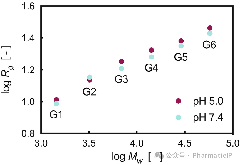
Fig. 2 Log-log plot of Rg calculated as a function of the PAMAM dendrimer molecular weight (Mw).
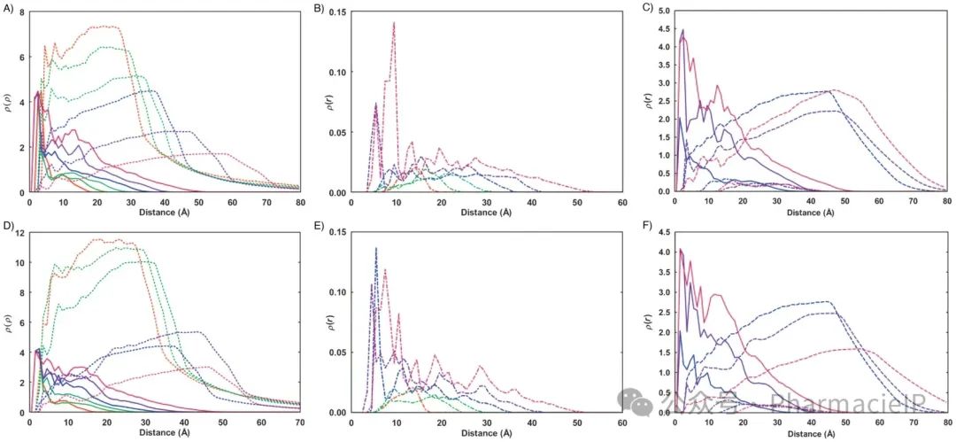
Fig. 3 Panels a, b, d, e: radial monomer distribution for G1 to G6 PAMAM dendrimers (continuous line), water (broken lines) and terminal nitrogens (dotted-broken lines) from MD simulations of each dendrimer in solution. Panels c and f: radial monomer distribution for G4 to G6 PAMAM dendrimers (continuous line) in complex with siRNA (dotted-broken lines) and water (broken lines). Results are from simulations at pH 5 (upper raw) and pH 7.4 (lower raw). Color code: red, G1; light green, G2; dark green, G3; blue, G4; purple, G5; dark red, G6.
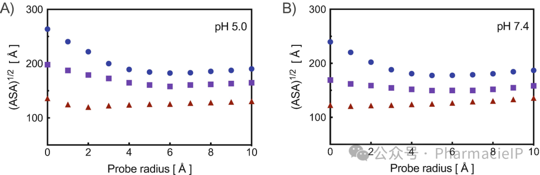
Fig. 4 Square root of the ASA as a function of the probe radius for PAMAM dendrimers G4 (blue circles), G5 (purple squares), and G6 (dark red triangles) at pH 5.0 (a) and pH 7.4 (b).
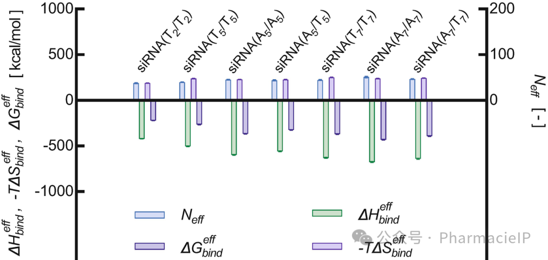
Fig. 5 G5 PAMAM dendrimer branches effectively interacting (Neff) involved in siRNA binding, as well as enthalpic (
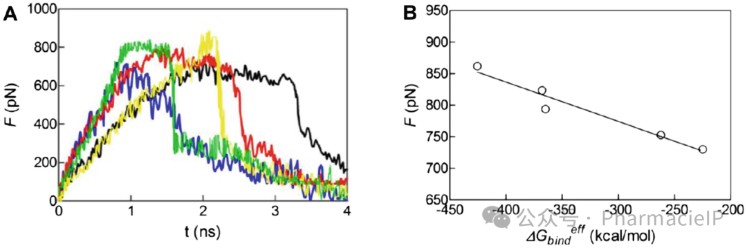
Fig. 6 (a) Time profile of the force of siRNA unbinding from their G% PAMAM dendrimer complexes. Color legend: blue, siRNA(T5/T5); green, siRNA(T7/T7)); yellow, siRNA(A7/A7)); red, siRNA(A5/A5)); black, siRNA(T2/T2). (b) Correlation between the CV-SMD peak force and the effective binding free energy