Abstract
Machine learning has become a mainstream solution applied across various industries. In this work, we investigate how to use side-channel information such as timing and electromagnetic (EM) emissions to perform reverse engineering of neural networks. To this end, we consider multilayer perceptrons and convolutional neural networks as the choices of machine learning architecture, assuming that non-invasive and passive attackers can measure these types of leaks.
We conducted all experiments on real data and commonly used neural network architectures. The experimental results indicate that side-channel attackers can obtain the following information: the activation functions used in the architecture, the number of layers and neurons in each layer, the number of output classes, and the weights in the neural network. Therefore, attackers can effectively reverse engineer the network using only side-channel information such as timing or EM emissions.
1 Introduction
This paper primarily studies two neural network algorithms: multilayer perceptrons (MLPs) and convolutional neural networks (CNNs). We consider feedforward neural networks, and thus our analysis is conducted only on such networks.
As the number of design strategies and elements to be used increases, tuning the hyperparameters of deep learning algorithms is becoming one of the main challenges. Essentially, the details are not disclosed when optimizing networks for commercial interests. Because these pre-trained models can provide additional information about the training data, this can be highly sensitive. For instance, if a model is trained based on patient medical records, confidential information can be encoded into the network during the training phase. Moreover, machine learning models used for medical guidance are often based on patients’ genotypes, which is very sensitive from a privacy perspective. Even if we ignore privacy issues.
Extracting useful information from neural network architectures helps gain commercial secrets from competitors, thereby producing competitive products without infringing intellectual property. So why would an attacker want to reverse engineer a neural network architecture rather than train the same network themselves? There are several reasons that complicate this approach. Firstly, attackers may not have access to the same training set to train their neural networks. Secondly, as architectures become increasingly complex, with more parameters to tune, it may be challenging for attackers to determine the same parameter values as those in the architecture of interest.
After motivating our use case, the main remaining question is the feasibility of reverse engineering such architectures. Physical access to the device can allow for easy reverse engineering based on binary analysis. However, in confidential IP settings, standard protections (such as preventing binary readback, blocking JTAG access, code obfuscation, etc.) are expected to be in place to prevent such attacks. A viable alternative is to exploit side-channel leaks.
In this work, we demonstrate the possibility of recovering unknown network layouts by leveraging side-channel information. Our approach does not require access to training data and allows for network recovery by feeding known random inputs into the network. By using known divide-and-conquer methods for side-channel analysis (i.e., the attacker’s ability to work with a manageable number of assumptions due to, for example, architectural details), information about each layer can be recovered. Thus, the recovered information can be used as input for recovering subsequent layers.
2 Background
2.1 Artificial Neural Networks
Artificial neural networks (ANNs) are a comprehensive concept for all computing systems, inspired by biological neural networks. Such systems can “learn” from examples, making them a powerful (and very popular) paradigm in the field of machine learning.
2.1.1 Multilayer Perceptron
A very simple neural network is called a perceptron. A perceptron is a linear binary classifier applied to feature vectors, serving as a function to determine whether an input belongs to a particular category. Perceptron classifiers are only applicable to linearly separable data, meaning that there exists a hyperplane that separates all positive points from all negative points. By adding more layers to the perceptron, we obtain the multilayer perceptron algorithm. A multilayer perceptron (MLP) is a feedforward neural network that maps input sets to appropriate output sets. It consists of multiple layers of nodes in a directed graph, where each layer is fully connected to the next layer. An MLP is composed of at least three layers: an input layer, an output layer, and one hidden layer. These layers must consist of nonlinear activation nodes.
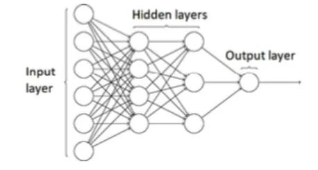
Figure 1: Multilayer Perceptron
2.1.2 Convolutional Neural Network
Convolutional neural networks represent a type of neural network originally designed for two-dimensional convolutions, inspired by biological processes in the animal visual cortex. CNNs use three main types of layers: convolutional layers, pooling layers, and fully connected layers. Convolutional layers are linear layers that share weights across space. Pooling layers are nonlinear layers that reduce spatial dimensions to limit the number of neurons. Fully connected layers are layers where each neuron is connected to all neurons in the neighboring layer.
2.1.3 Activation Functions
The activation function of a node is defined as the output function f of the node given an input or a set of inputs. Nonlinear activation functions are required to compute some unusual functions of ANNs using a minimal number of nodes.

This paper considers the Logistic (Sigmoid) function, Tanh function, Softmax function, and Rectified Linear Unit (ReLU) function.
2.2 Side-Channel Analysis
Side-channel analysis (SCA) exploits vulnerabilities at the implementation level. More specifically, all computations running on a platform lead to unintended physical leaks, which are physical signatures from response times, power consumption, and electromagnetic (EM) radiation released when the device processes data. SCA utilizes these physical signatures to recover keys (secret data). In its basic form, SCA is proposed to perform key recovery attacks on cryptographic implementations. One advantage of SCA over traditional cryptanalysis is that SCA can apply divide-and-conquer methods. This means that SCA typically recovers a small portion (subkey) of the key one at a time, reducing the complexity of the attack.
Simple Power (or Electromagnetic) Analysis (SPA or SEMA). Simple power (or EM) analysis, as the name suggests, is the most basic form of SCA. Its goal is to extract information from sensitive computations that can be recovered from a single or a few traces. A common example is that SPA can be used against the direct implementation of the RSA algorithm to distinguish between squaring and multiplication operations, thereby achieving key recovery. In this work, we apply SPA, or rather SEMA, to reverse engineer the architecture of neural networks.
Differential Power (or Electromagnetic) Analysis (DPA or DEMA). DPA or DEMA is an advanced form of SCA that applies statistical techniques to recover confidential information from physical signatures. The attack typically tests the correlation between actual physical signatures (or measurements) and assumed physical signatures (i.e., predictions of intermediate data). The assumed signatures are based on leakage models and key hypotheses. A small portion of the key (e.g., one byte) can be tested independently. Knowledge of the leakage model comes from expert intuition and expertise. In the following, we use DPA (DEMA) to recover secret weights from a pre-trained network.
3 Side-Channel-Based Neural Network Reverse Engineering
In this section, we will discuss the threat model we used, the experimental setup, and the reverse engineering of various elements of the neural network.
3.1 Threat Model
We chose to work with MLPs and CNNs because 1) they are commonly used machine learning algorithms in modern applications; 2) they consist of different types of layers that also appear in other architectures, such as recurrent neural networks; and 3) in the case of MLPs, the layers are all the same, making SCA more challenging and thus can be considered the worst-case scenario.
We chose to make our attack as general as possible. For example, when dealing with real numbers, we make no assumptions about the type or source of the input. If the input is in integer form (e.g., the MNIST database), the attack becomes easier since we do not need to recover tail bytes and handle precision. We also assume that the implementation of the machine learning algorithm does not include any side-channel countermeasures.
Capabilities of the attacker: 1. The attacker does not know the architecture of the network used but can provide random (thus known) inputs to that architecture. We assume the attacker can physically access the device (which can be accessed remotely via EM signals) and knows that the device runs some neural network. The attacker controls its execution merely by selecting inputs, but he/she can observe outputs and side-channel information (but not isolated intermediate values). 2. The attacker is able to measure side-channel information leaked from the implementation of the target architecture. The attacker can collect multiple side-channel measurements while processing data and analyze them using different side-channel techniques. In this work, we mainly focus on timing and EM side channels.
3.2 Experimental Setup
Here, we describe the attack method first validated on the Atmel ATmega328P. Subsequently, we also demonstrate the proposed method on the ARM Cortex-M3.
Side-channel activities are captured using a LeCroy Waverunner 610ZI oscilloscope. For each known input, the attacker obtains a measurement (or trace) from the oscilloscope. In the following, the interchangeability of input or NR. traces will be used. Each measurement consists of several samples. The number of samples (or trace length) depends on the sampling frequency and execution time. As shown later, depending on the target, the number of NR. samples can range from thousands (multiplicative) to millions (entire CNN network). The measurements are synchronized with operations through common handshake signals, such as the start and stop of computation. To further improve measurement quality, we mechanically opened the chip package (see Figure 2a). An RF-U5-2 near-field electromagnetic probe from Langer is used to collect electromagnetic measurements (see Figure 2b). The setup is shown in Figure 2c. We use the probe as an antenna to monitor EM side-channel leaks from the underlying processor running ML. Note that EM measurements also allow for observing the timing of all operations, thus this setup also allows for timing side-channel analysis.
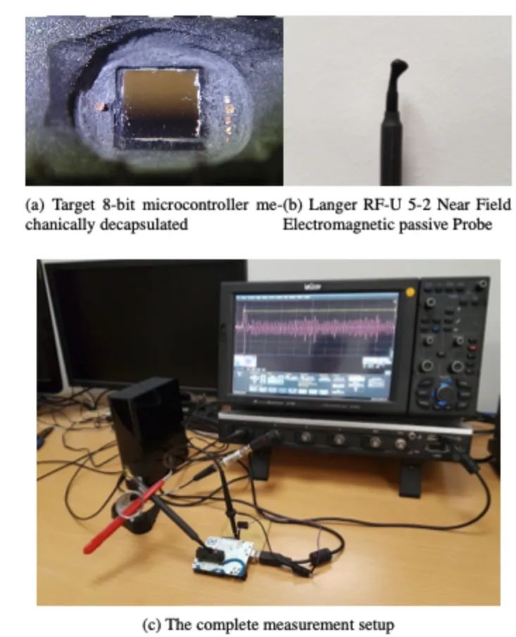
Figure 2: Experimental Setup
As mentioned above, the leakage model for the developed target device is the Hamming Weight (HW) model. The microcontroller loads sensitive data onto the data bus to execute the indicated instruction. Before each instruction, the data bus is precharged to all “0”. Note that the precharging of the data bus is a natural behavior of the microcontroller and is not a vulnerability introduced by the attacker. Thus, the power consumption (or EM radiation) allocated to the value of the data being loaded is modeled as the number of bits equal to “1”.
Several pre-trained networks are installed on the board. The training phase is conducted offline, then the trained network is implemented in C language and compiled on the microcontroller. In these experiments, we consider multilayer perceptron architectures composed of different numbers of layers and nodes within those layers. Note that using our method, there is no limit to the number of layers or nodes we can attack, as the attack scales linearly with the size of the network. The method demonstrates that key parameters of the network, namely weights and activation functions, can be reverse-engineered. Further experiments were conducted on a deep neural network with three hidden layers, but the method remains effective for larger networks.
3.2 Reverse Engineering Activation Functions
To represent nonlinear functions with a small number of nodes in the network, nonlinear activation functions are necessary. Therefore, they are components used in almost all neural network architectures today. If the attacker can infer information about the type of activation function used, he/she can use that knowledge along with information about the input values to infer the overall behavior of the network.
We analyzed the side-channel leaks of different activation functions. We considered the most commonly used activation functions, namely ReLU, Sigmoid, Tanh, and SoftMax. Timing behavior can be directly observed on the EM traces.
We tested different variants with each activation function. We collected EM traces and measured the time taken for the activation function computation based on the measurement results. Measurements were taken when the network processed random inputs within the range, i.e., x∈{−2,2}. A total of 2000 EM measurements were captured for each activation function. As shown in Figure 3, the timing behaviors of the four tested activation functions exhibit different characteristics, allowing for easy characterization.
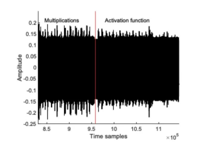
Figure 3: Observed Patterns and Timing of Multiplication and Activation Functions
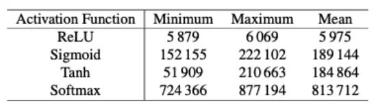
Different inputs lead to different processing times. Additionally, the timing behavior for the same input varies significantly depending on the activation function. For example, we can observe that due to its simplicity, ReLU requires the shortest time (see Figure 4a). In contrast, Tanh and Sigmoid may have similar timing delays, but they exhibit different patterns depending on the input (see Figures 4b and 4c), where Tanh is more symmetrical in pattern than Sigmoid for positive and negative inputs. We can observe that the softmax function requires most processing time as it involves exponentiation, which also depends on the number of neurons in the output layer. Since neural network algorithms are typically optimized for performance, the presence of such timing side channels is often overlooked. Functions like Tanh or Sigmoid require computations of Ex and division, and it is known that such functions are difficult to implement in constant time. Thus, constant-time implementations may lead to significant performance degradation. Other activation functions can similarly be characterized. Table 1 shows the minimum, maximum, and average computation times for each activation function across 2000 captured measurements. While ReLU is the fastest, the time differences for other functions are significant enough to allow for direct recovery. To distinguish them, pattern matching can also be performed if necessary to determine which type of function is used. Moreover, attackers can sometimes pre-describe the timing behavior of the target activation function to achieve better accuracy, especially when standard libraries are used for standard functions (like multiplication, activation functions, etc.).
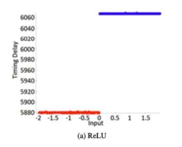
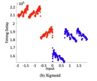
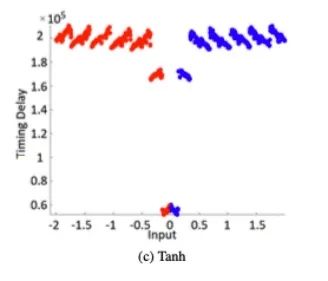
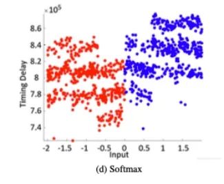
Figure 4: Timing Behavior of Different Activation Functions
Table 1: Minimum, Maximum, and Average Computation Times for Different Activation Functions
3.4 Reverse Engineering Multiplication Operations
By fine-tuning the weights, we can improve the accuracy of the network. Below, we will demonstrate a method for recovering these weights using SCA.
We start by analyzing how the compiler handles floating-point operations for our target processor. The generated components are shown in Table 2, confirming the use of the aforementioned IEEE754 compatible representation. Since the target device is an 8-bit microcontroller, the representation follows a 32-bit pattern (b31,…,b0), stored in 4 registers. The 32 bits include: 1 sign bit (b31), 8 biased exponent bits (b30,…,b23), and 23 mantissa (fraction) bits (b22,…,b0). It can be expressed as:
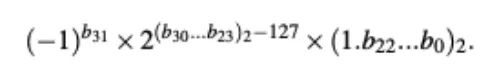
When the computed result m is stored back to memory, consider measuring t in the HW model’s leakage, i.e., HW(m). Since 32-bit m is split into individual 8 bits, each byte of m can be recovered individually. Thus, by recovering this representation, it is sufficient to recover an estimate of the real number value.
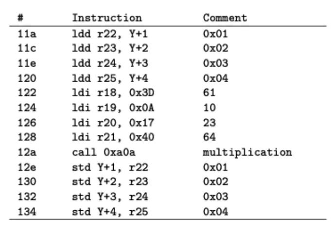
Table 2: Code Snippet for Returning Assembly Used for Multiplication: X=XW(=2.36 or 0x3D0A1740 in IEEE754 representation). The multiplication itself is not shown here, but our leakage model holds based on the register allocation.
To implement the attack, two different approaches can be used. The first approach is to establish hypotheses based on direct weights. For this experiment, we target the product m of known input value X and unknown weight w. For each input, we assume different possibilities for the weight value. We then perform multiplication and estimate the output’s IEEE754 binary representation. We then proceed to recover the 23-bit mantissa of the weight. The sign and exponent can be recovered separately. Therefore, we are observing the leakage of 3 registers, and based on the best CPA results for each register, we can reconstruct the mantissa.
In Figure 5, we show the correlation results for each byte with the measurement traces. The x-axis represents execution time, and the y-axis represents correlation. Each case was tested with 1000 traces. In the figure, the black curve represents the correlation coefficient while the red area comes from all other candidate weights within that range.
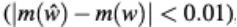
Figure 5: Correlation of Different Weight Candidates in Multiplication Operations
3.5 Reverse Engineering the Number of Neurons and Layers
After recovering the weights and activation functions, we now use SCA to determine the structure of the network. Primarily, we are interested in seeing if we can recover the number of hidden layers and the number of neurons in each layer. To perform the reverse engineering of the network structure, we first use SPA (SEMA). SPA is the simplest form of SCA, allowing the recovery of information in a single (or few) traces through simple visual inspection methods. Analyzing an MLP with 6 neurons in the hidden layer corresponds to the EM traces for processing random inputs as shown in Figure 6a. By observing the EM traces, it is easy to compute the number of neurons. The observability stems from the multiplication operations and activation functions (in this case, it is the Sigmoid function) having entirely different leakage characteristics. Similarly, the structure of deeper networks is also illustrated in Figures 6b and 6c. The recovery of the output layer provides information about the number of output classes.
However, distinguishing different layers may be difficult, as the leakage patterns depend only on the multiplication and activation functions that typically exist in most layers. We observed secondary features that allow for identifying layer boundaries, but with low confidence. Therefore, we developed a different CPA-based method to identify layer boundaries.
Let us assume our target is the first hidden layer (the same method can also be applied to different layers). Assume the input is a vector of length N0, so the input X can be represented as x={x1,…,xN0}. For the target neuron yn in the hidden layer, weight recovery is performed based on two different hypotheses. For the first hypothesis, assume that yn is in the first hidden layer. Weight recovery is performed using Xi (1≤i≤N0) individually. For the second hypothesis, assume that yn is in the next hidden layer (the second hidden layer). Weight recovery is performed using yi individually for 1≤i≤n-i. For each hypothesis, the maximum (absolute) correlation value is recorded and compared between the two. Since correlation depends on two inputs from multiple inputs, in iterative operations, incorrect hypotheses will lead to lower correlation values. Thus, this can be used to identify layer boundaries.
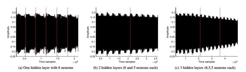
Figure 6: SEMA on Hidden Layers
3.5 Full Network Layout Recovery
The combination of the various techniques developed earlier can subsequently lead to the complete reverse engineering of the network. Complete network recovery is performed layer by layer, and for each layer, the weights of each neuron must be recovered one at a time. Let us consider a network composed of N layers L0, L1, …, LN−1, where L0 is the input layer and LN−1 is the output layer. The steps to perform reverse engineering are as follows:
1. The first step is to recover each connected weight WL0 from the input layer (L0) to the first hidden layer (L1). Since the size of the input layer is known, CPA/CEMA can be performed NL0 times (the size of L0). For 2^d hypotheses (D is the number of bits in the IEEE754 representation, usually 32 bits, but for simplicity, 16 bits can be used for lower mantissa precision), correlation is computed. After the weights are recovered, the output of the multiplication and summation can be computed. This information provides us with the input for the activation function.
2. To determine the output of the multiplication and summation, the number of neurons in the layer must be known. This can be recovered using a combination of the SPA/SEMA and DPA/DEMA techniques described in the previous subsection, paralleling the recovery of weights. When all weights of the first hidden layer are recovered, the following steps are executed.
3. Using the same set of traces, timing patterns for different inputs to the activation functions can be constructed, similar to Figure 4. The timing patterns or average timings can then be compared with profiles of each function to determine the activation function (the comparison can be based on simple statistical tools such as correlation, distance metrics, etc.). The output of the activation function can then be computed, which will provide input to the next layer.
4. In subsequent layers (L1,…,LN−1, thus up to a total of 2N_(nL)2*d), the same steps are repeated until the entire network structure is recovered.
4 Experiments with ARM Cortex-M3
In this section, we will extend the existing attacks on 32-bit ARM microcontrollers. The measurement setup is similar to previous experiments (Langer’s LeCroy Waverunner 610ZI oscilloscope and RFU5-2 near-field electromagnetic probe). Measurement points are determined by benchmark code running AES encryption. After capturing the measurements of the target neural network, reverse engineering can be performed.
The timing behaviors of various activation functions are shown in Figure 7. While this result differs from previous experiments on AVR, it exhibits unique timing characteristics that allow for the identification of each activation function. The activity of a single neuron is shown in Figure 8a, which uses Sigmoid as the activation function (multiplication operations are separated by vertical red lines). Figure 8b shows a successful attack recovering the secret weight of 2.453 under known input conditions. As previously mentioned, side-channel measurements on modern 32-bit ARM Cortex-M3 may have lower SNR, making the attack more challenging. Nevertheless, even with more than two measurements on ARM, this attack has proven feasible. In our setup, conducting 200 additional measurements takes less than a minute. Similarly, measurement setups and quantities can be updated for other targets (such as FPGA, GPU, etc.).
Finally, the complete neural network is recovered. The state of the entire network is shown in Figure 8c. All neurons can be visually observed. The determination of layer boundaries (indicated by red solid lines) can be established through multiplication operations.
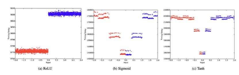
Figure 7: Timing Behavior of Different Activation Functions
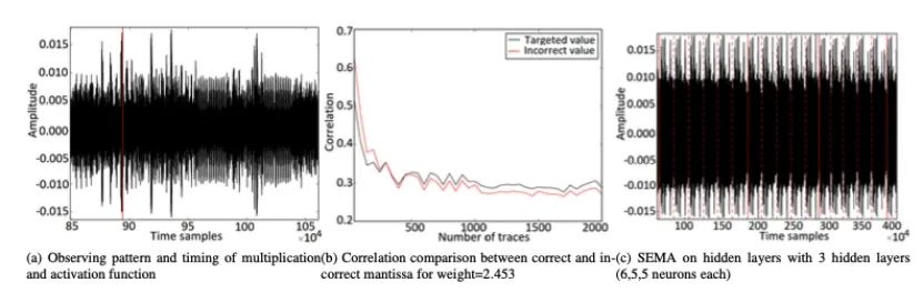
Figure 7: Analysis of Neural Network (6,5,5)
5 Further Discussion and Conclusion
In this work, we have practically demonstrated the reverse engineering of neural networks using side-channel analysis techniques. Specific attacks are performed on measurement data corresponding to the implementation of the chosen network. To make our setup more general, we do not assume any specific form of input data (other than that the input is real-valued).
We conclude that with an appropriate combination of SEMA and DEMA techniques, all sensitive parameters of the network can be recovered. The proposed method has been demonstrated on two different modern controllers, one being the classic 8-bit AVR and the other the 32-bit ARM Cortex-M3 microcontroller. In the current experiments, the attacks required double the measurements, taking approximately 20 seconds of overtime. Overall, the attack method scales linearly with the size of the network. In certain setups where new networks are derived from known networks such as VGG-16, AlexNet, etc., the attack may be easier. By adjusting hyperparameters or transfer learning. In such cases, side-channel methods can reveal remaining secrets. However, the analysis of such partial cases is currently out of scope.
Acknowledgments
This paper is translated and summarized by Liu Fan, a master’s student of the 2021 class at the School of Software, Nanjing University.