Translator | Zhu Xianzhong

Reviewer | Liang Ce, Sun Shujuan

Abstract:This article will provide some background knowledge on methods for image recovery tasks, aiming to help readers create a similar image search engine for specific goals (excluding the development of complete enterprise solutions).

Main Text:

Project Overview

Similar image retrieval is any image-related search, known as “content-based image retrieval system”, abbreviated as “CBIR” system.

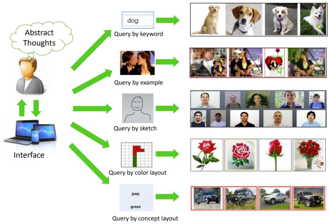
The above image is from the article “Content-Based Image Retrieval: A Comprehensive Literature Survey (2017)” (https://arxiv.org/abs/1706.06064)

Today, the application of image search is becoming increasingly widespread, especially in the field of e-commerce services (such as AliExpress, Wildberries, etc.). “Keyword search” (including image content understanding) has long established itself in search engines like Google and Yandex, but its application in markets and other private search engines is still relatively limited. The introduction of the contrastive language-image pre-training CLIP (https://openai.com/blog/clip/) in the field of computer vision has caused a sensation and will accelerate its globalization.

Our team specializes in neural networks in computer vision, so in this article, I will focus on introducing methods for image search.

1. Basic Service Components

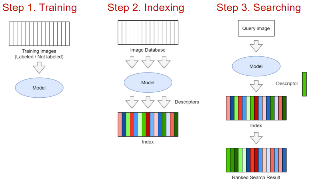
Step 1: Train the Model. The model can be established based on classical computer vision or neural network foundations. The input part of the model is an image, and the output part is a D-dimensional descriptor/embed layer. In classical implementations, a strategy combining SIFT (Scale-invariant feature transform) descriptors and BoW (bag-of-visual-words) algorithms can be used. However, in neural network implementations, standard algorithm models (such as ResNet, EfficientNet, etc.) can be combined with complex pooling layers and further enhanced by excellent learning techniques. If the data is sufficient or well-trained, choosing the neural network solution will almost always yield satisfactory results (proven by personal tests), so we will focus on this solution in this article.

Step 2: Index the Images. This step involves running the trained model on all images and writing the embeddings into a special index for rapid searching.

Step 3: Search. Use the user-uploaded image, run the model, obtain the embedding layer, and compare it with other embedding data in the database. The final search results are sorted by relevance.

2. Neural Networks and Metric Learning

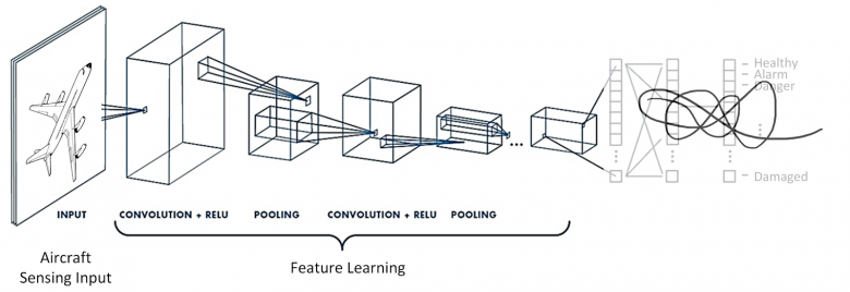
In tasks of finding similarities, we use neural networks as feature extractors (backbone networks). Of course, the choice of the backbone network depends on the capacity and complexity of the data—you can choose from various options ranging from ResNet18 residual networks to Visual Transformer models based on your development needs.

The first feature of the image retrieval model is the implementation technology of the output part of the neural network. In the image retrieval leaderboard (https://kobiso.github.io/Computer-Vision-Leaderboard/cars.html), different image retrieval algorithms aim to construct the most ideal descriptors—for instance, there are algorithms using combined global descriptors with parallel pooling layers, and batch deletion block algorithms that achieve a more uniform activation distribution in the output function.

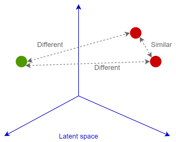
The second main feature is the loss function. Currently, there are many loss functions in the field of artificial intelligence. For example, in the paper “Deep Image Retrieval Survey” (https://arxiv.org/abs/2101.11282), more than a dozen recommended loss function algorithms are mentioned. There are also a considerable number of classification functions. The primary goal of all these loss functions is to train the neural network to convert images into linearly separable spatial vectors, allowing for further comparison of these vectors using cosine or Euclidean distance: similar images will have similar embedding layers, while dissimilar images will have vastly different embedding layers. Next, let’s further introduce these contents.

Loss Functions

1. Contrastive Loss

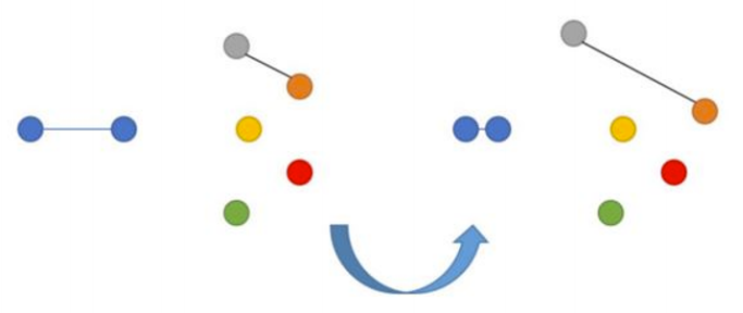
This algorithm presents a dual loss situation, often occurring when comparing the distances between objects.

If images p and q are indeed very similar, the neural network will be penalized for the distance between the embedding layers of images p and q. Similarly, due to the proximity of the embedding layers, the neural network may also face penalties when the embedding layers of the images are actually different. In the latter case, we can set a margin value m (for instance, set to 0.5) to overcome the assumption that the neural network has already handled the task of “separating” dissimilar images.

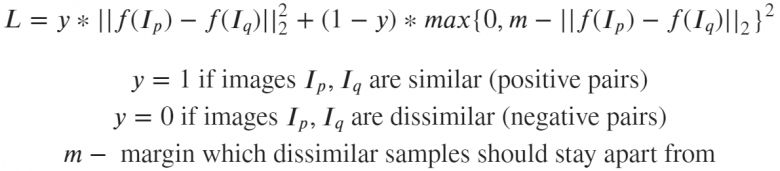
2. Triplet Loss

Here, our goal is to minimize the distance from the anchor to the positive example while maximizing the distance from the anchor to the negative example. The triplet loss function was first seen in Google’s FaceNet model regarding face recognition and has long been a state-of-the-art solution.

3. N-tupled Loss

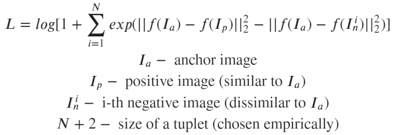
The N-tupled loss function is a further study based on the triplet loss function. This function also adopts the concepts of anchors and positive examples but uses multiple rather than single negative examples.

4. Angular Additive Margin Loss (also known as ArcFace)

The problem with paired loss functions lies in the combination of positive examples, negative examples, and anchors—if they are merely selected uniformly at random from the dataset, a “light pairing” issue arises. In such straightforward image pairings, the loss is zero. It turns out that in this scenario, the network quickly converges to a state where most elements in the batch are easy to handle, and their losses become zero—at this point, the neural network stops learning. To avoid this issue, developers of this algorithm began proposing complex pairing mining techniques—hard negative mining and hard positive mining. For related issues, refer to (https://gombru.github.io/2019/04/03/ranking_loss/), which compares various loss functions. Additionally, the PML library (https://github.com/KevinMusgrave/pytorch-metric-learning) implements many mining methods. Notably, this library contains a wealth of useful information for metric learning tasks in the PyTorch framework.

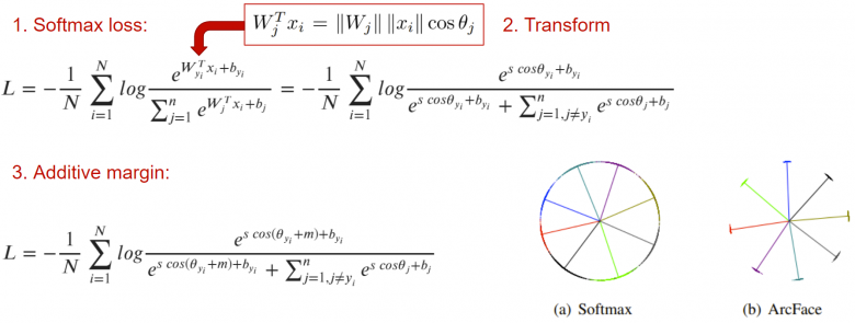
Another solution to the aforementioned problem is to use classification loss functions. Let’s recall the facial recognition algorithm ArcFace, which was launched three years ago and was the state-of-the-art at the time, leading to the well-known “defective” features.

The main idea of this algorithm is to add an indentation m to the usual cross-entropy, where this cross-entropy distributes the embedding layers of a class of images around the centroid area of that class, ensuring that they are at least separated by an angle m from the embedding layers of other classes.

This seems to be a perfect solution for a loss function, especially when developing AI systems for the MegaFace benchmark (https://paperswithcode.com/sota/face-verification-on-megaface) scale. However, it is important to remember that this algorithm only works when classification labels are present; otherwise, you will face the issues of paired loss functions.

The above image visually demonstrates which loss functions are most suitable when using single-class labels and multi-class labels (you can derive paired labels from multi-class labels by calculating the percentage of intersection between multi-label vector samples).

Pooling

Now, let’s review the neural network architecture, considering the case of using a pair of pooling layers in performing image retrieval tasks.

1. R-MAC Pooling

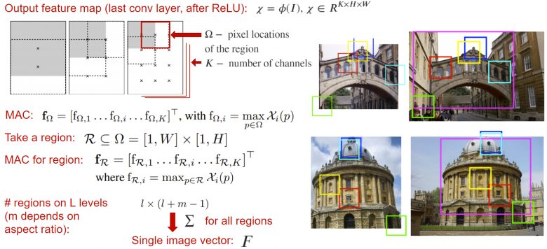
R-MAC (Region-based Max Pooling) is a pooling layer that accepts the output maps of the neural network (before the global pooling layer or classification layer) and returns a descriptor vector that is the sum of the activation amounts in each window within the output image. Here, the activation amount of the window is taken as the maximum value obtained for that window in each channel.

This resulting descriptor is calculated considering the local features of the image at different scales, thereby creating a rich content feature description. This descriptor itself can be an embedding layer and can thus be directly sent to the loss function.

2. GeM Pooling

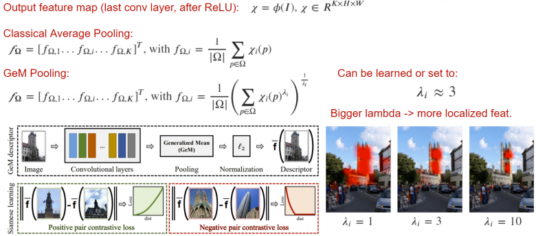
GeM (Generalized Mean Pooling) is a simple pooling algorithm that can improve the quality of output descriptors. The bottom line is that classical average pooling can be generalized to the lambda norm. By adding a lambda layer, we enable the neural network to focus on important parts of the image, which may be crucial in certain tasks.

Distance Measurement

1. Indexing

The key to high-quality search for similar images is ranking, which displays the most relevant samples for a given query. The basic features of this process include the speed of establishing descriptor indexes, the speed of searching, and the memory occupied.

The simplest method is to keep the embedding layers “facing forward” and conduct a strong search using cosine distance. However, this method encounters problems when there are a large number of embedding layers—potentially millions, tens of millions, or more. Moreover, the search speed significantly decreases, and the occupied heap space further increases. However, there are positive aspects—using existing embedding layers can achieve perfect search quality.

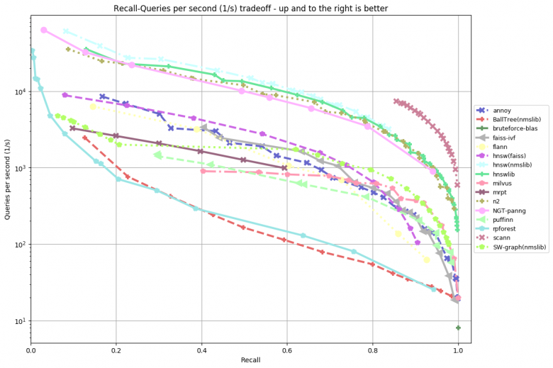
These issues can be resolved at the cost of quality—by compressing (quantizing) rather than storing the embedding layers in their raw form. Additionally, the search strategy needs to be altered—not using brute-force search, but attempting to minimize the number of comparisons needed to find the closest comparisons to the given query. Currently, there are many effective search frameworks available for approximate nearest neighbor search. To achieve this, a special benchmark has been created—based on this benchmark, you can observe the performance of each library on different datasets.

Among the most popular libraries are: NMSLIB (Non-Metric Space Library), Spotify’s Have Library, Facebook’s Faiss Library, and Google’s Scann Library. Additionally, if you want to index using a REST API, you can consider using the Jina application (https://github.com/jina-ai/jina).

2. Re-ranking

Researchers in the field of information retrieval have long understood that after receiving the original search results, some means of reordering the items can improve the ordered search results.

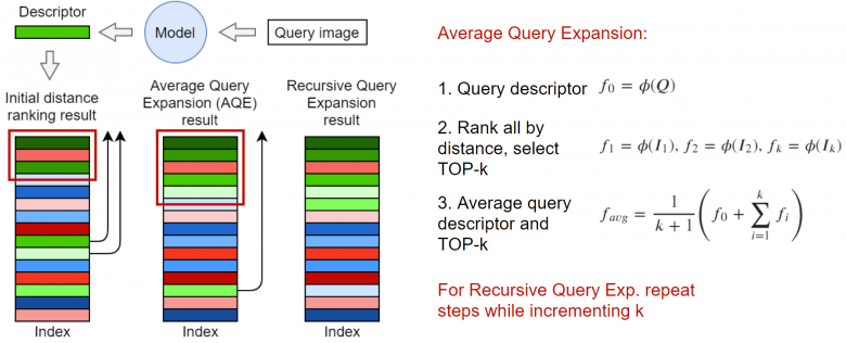
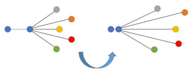
A well-known algorithm is Query Expansion. The core idea of this algorithm is to generate new embeddings using the top-K closest elements in the set. In the simplest case, the average vector can be taken as shown in the figure above. In fact, you can also perform weighted operations on the embeddings based on the distance in the problem or the cosine distance with the request. The framework detailed in the paper “Attention-Based Query Expansion Learning” (https://arxiv.org/abs/2007.08019) mentions this in detail, or you can recursively use the query expansion algorithm.

3. k-Nearest Neighbors Algorithm

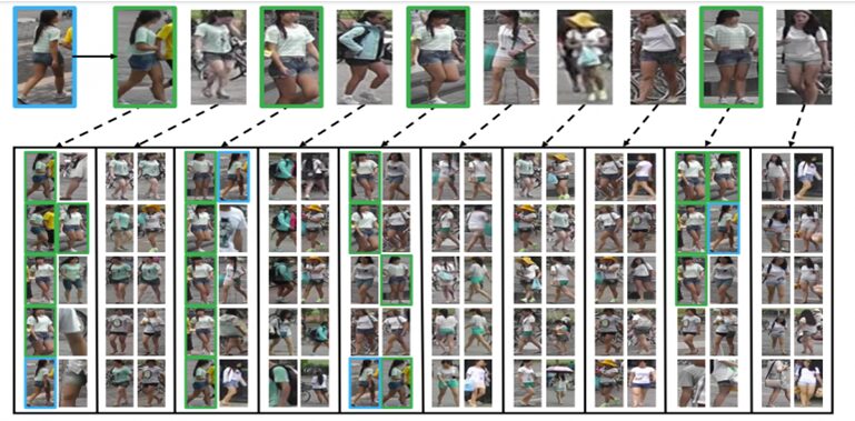
The image above is a screenshot of an application for identifying the nearest objects to a person. The top of the image shows the query and its 10 nearest neighbor data, where P1-P4 are positive examples, and NI-N6 are negative examples. The bottom of the image shows the 10 nearest neighbors for the sample person in each of the two columns. The blue and green boxes correspond to the sample person and positive examples, respectively. We can observe that the sample person and positive examples have 10 nearest neighbors among each other.

The k-nearest neighbors algorithm primarily revolves around the top-k elements, which include the k elements closest to the request itself.

Based on this set, a reordering process is established, which is described in the paper “Research on Person Re-identification Information Reordering Based on k-Nearest Neighbors Algorithm” (https://arxiv.org/abs/1701.08398). By definition, the k-reciprocal algorithm is closer to the query results than the k-nearest neighbors algorithm. Therefore, one can roughly consider that the elements in the k-nearest neighbors algorithm set are positive examples, and further change the weighting rules for algorithms similar to query expansion.

In this paper, a mechanism has been developed that can recalculate distances using the k-nearest neighbor set of elements from the top-k itself. This paper contains a wealth of computational information that is temporarily outside the scope of this discussion; interested readers are encouraged to read it independently.

Analysis of Similar Image Search Algorithm Effectiveness

Next, let’s analyze the quality issues of the similar image search algorithm proposed in this article. It is worth noting that there are many details in the implementation of this search task, which beginners are likely to overlook when developing image retrieval projects for the first time.

1. Metrics

This article will explore some popular metric algorithms commonly used in the field of image retrieval, such as precision@k, recall@k, R-precision, mAP, and nDCG, etc.

[Translator’s Note]Generally speaking, precision in the algorithms mentioned below represents how many of the retrieved items are accurate, while recall represents how many of all accurate items are retrieved.

(1) Precision@R Algorithm

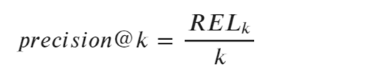
In the above formula,

the parameter REL_k represents: the number of relevant samples in the top-k results;

the parameter k represents: the fixed number of top positions to be considered.

Advantages: It can display the percentage of relevant samples in the top-k.

Disadvantages:

• Very sensitive to the number of relevant samples for a given query, which leads to an inability to objectively assess search quality since the number of relevant samples varies across different queries.
• Can only achieve a value of 1 when the number of relevant samples in all queries is greater than or equal to k.

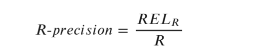
(2) R-Precision Algorithm

In the above formula,

the parameter REL_R represents: the number of relevant samples in the top-R results;

the parameter R represents: the number of all relevant samples in the given query.

Similar to the precision@k algorithm, the parameter k is also set to the number of relevant query samples.

Advantages: Unlike the sensitivity of the number k in precision@k, the metric becomes stable.

Disadvantages: It is necessary to know the total number of samples relevant to the request in advance (if not all relevant numbers are labeled beforehand, it may cause problems).

(3) Recall@k Algorithm

In the above formula,

the parameter REL_k represents: the number of relevant samples in the top-k results;

the parameter k represents: the fixed number of top positions to be considered;

the parameter REL represents: the number of all relevant samples in the given query.

This algorithm can display the proportion of relevant sample items found in the top-k.

Advantages:

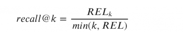
• Answers whether relevant items are present in the top-k.
• Stable and averages over requests.

(4) mAP (Mean Average Precision) Algorithm

This algorithm can show the density of relevant samples at the top of search results. You can think of it as the amount of information received by search engine users, with the minimum number of pages read by the search engine. Therefore, the greater the ratio of information to the number of pages read, the higher the metric.

Advantages:

• Provides an objective and stable assessment of search quality.
• A single-digit representation of the precision-recall curve, which carries rich analytical information.

Disadvantages:

• Must know the total number of samples relevant to the request (if not all relevant samples are labeled beforehand, it may cause problems).

[Tip] More information about the mAP algorithm output can be found in https://nlp.stanford.edu/IR-book/html/htmledition/evaluation-of-ranked-retrieval-results-1.html.

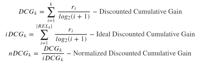
(4) nDCG (Normalized Discounted Cumulative Gain) Algorithm

In the above formula,

the parameter REL_k represents: the list of relevant samples before position k (sorted by relevance);

the parameter r_i represents: the rounded true relevance score of the i-th item in the retrieval results.

This metric algorithm shows how well the elements in the top-k are ordered among themselves. Since this is the only metric algorithm that considers the order of elements among the above methods, we will not elaborate on its advantages and disadvantages. However, research has shown that when order matters, this metric algorithm is quite stable and applicable in most cases.

2. Overall Estimation of the Algorithm

(1) Macroscopic: Calculate a metric for each request and compute the average across all requests.

• Advantages: There is no significant fluctuation in the number of data relevant to this query.

• Disadvantages: All queries are treated as equivalent, although some queries are more relevant than others.

(2) Microscopic: Sum the number of marked relevant items and those successfully found as relevant across all queries, and then include them in the calculation of the corresponding metric.

• Advantages: When evaluating queries, it considers the number of marked items relevant to each query.

• Disadvantages: If a request has many marked relevant metrics and the system fails to bring them to the top, the metric calculation results may become very low or very high.

3. System Validation

Readers are advised to adopt the following two validation schemes for the algorithm proposed in this article:

(1) Validation Based on a Set of Queries and Selected Relevant Queries

Input: Image requests and related images, with a list of relevant items associated with this query.

To calculate metrics, a relevance matrix can be computed for each element, based on the binary information of element relevance.

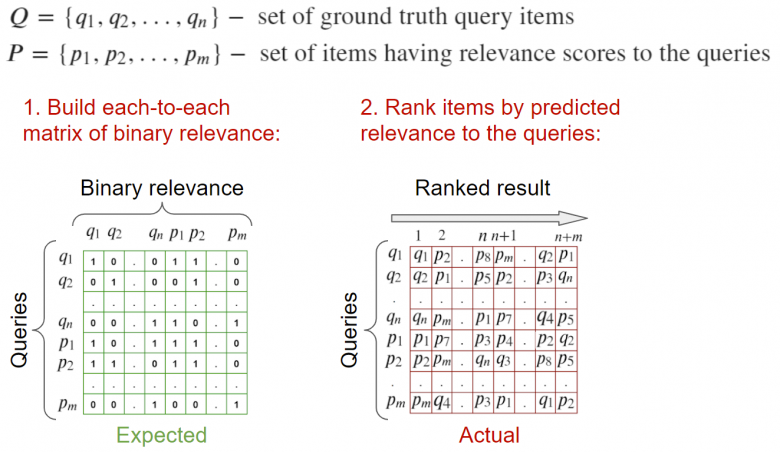
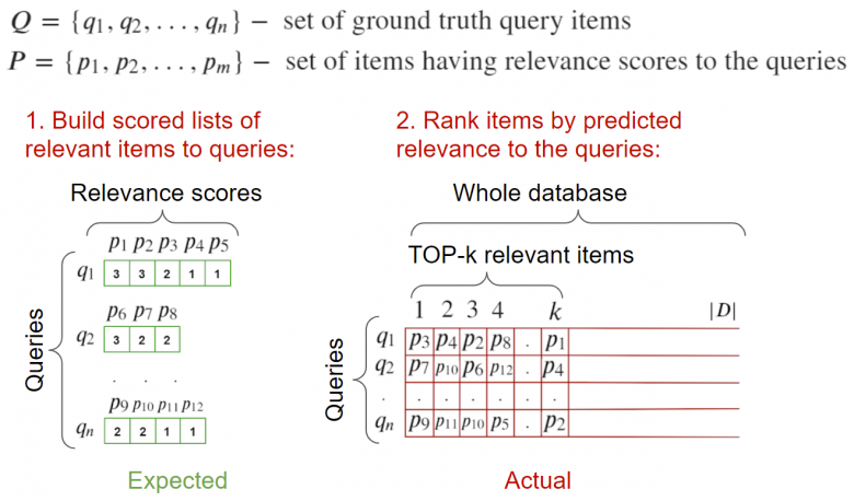
2. Full Base Validation

The input part of this algorithm includes: image requests and related images, along with an image validation database—ideally, all relevant queries should be marked within it. Moreover, the database should not include the query images; otherwise, such images would need to be cleaned during the search phase to avoid blocking the top-1 layer. Additionally, a set of negative examples is provided as a validation base—our task is to find relevant items.

To calculate metrics, you can traverse all requests, compute the distances to all elements (including relevant ones), and then send them to the metric calculation function.

Completed Project Examples

In the question of whether a company should use another brand’s graphic elements, disputes often arise between companies. In such cases, weaker manufacturers attempt to parasitize a successful major brand by displaying similar symbols for their products and services. However, consumers are also affected— you may want to buy cheese from a trusted manufacturer but fail to read the label carefully, thus mistakenly purchasing inferior products from a counterfeit manufacturer. A recent case involved Apple attempting to block Prepear’s logo trademark usage (https://www.pcmag.com/news/apple-is-attempting-to-block-a-pear-logo-trademark).

As a result, some professional governmental organizations or private companies are working to combat illegal transplantation. They hold a registry of registered trademarks, through which they can compare upcoming trademarks and ultimately decide whether to approve or reject trademark registration applications. The above is a typical example of using the WIPO (https://www3.wipo.int/branddb/en/) system interface, where the search for similar image functionality will greatly facilitate the work of relevant experts in quickly searching for similar images.

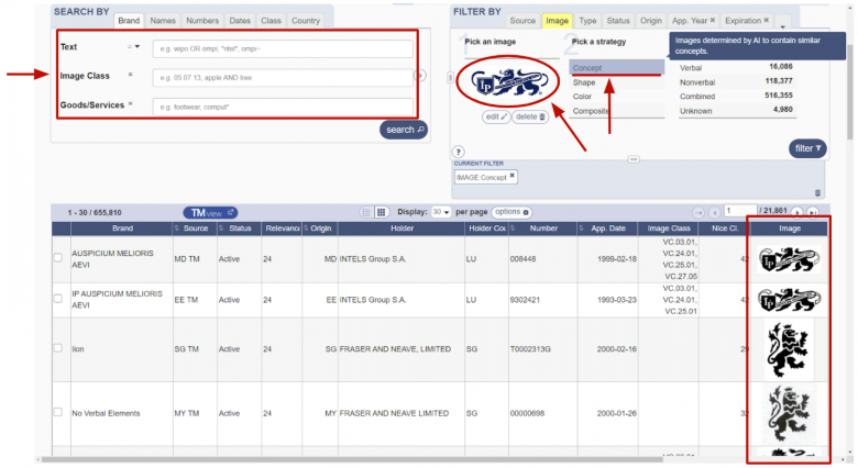
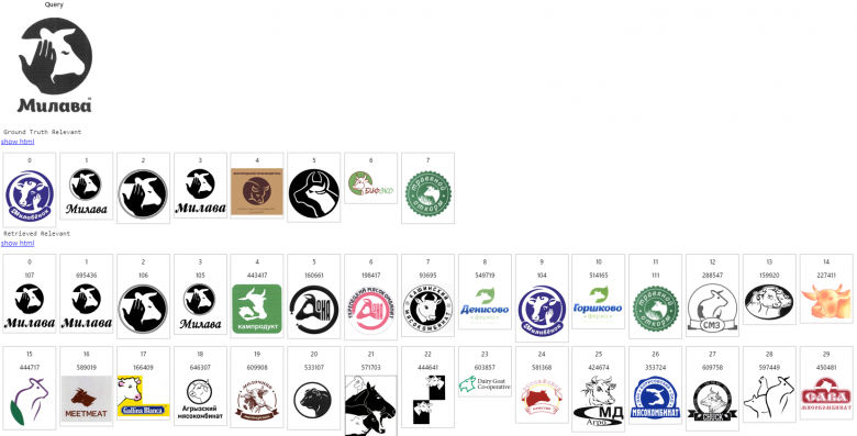
1. System Application Example

In the system we developed, the indexed image database contains millions of trademarks. The first image provided is a query result display, the next line (the second image) gives a list of expected relevant images, and the remaining images in the following rows are search results provided by the search engine in descending order of relevance.

Translator Introduction

Zhu Xianzhong, 51CTO community editor, 51CTO expert blogger, lecturer, computer teacher at a university in Weifang, a veteran in the programming world. Early on focused on various Microsoft technologies (authored three technical books related to ASP.NET AJX, Cocos 2d-X), and has spent the last decade in the open-source world (familiar with popular full-stack web development technologies), understanding IoT development technologies based on OneNet/AliOS + Arduino/ESP32/Raspberry Pi and big data development technologies like Scala + Hadoop + Spark + Flink.

Original link:

https://hackernoon.com/how-to-build-an-image-search-engine-to-find-similar-images

Community Editor Recruitment

51CTO sincerely invites you to join the community editor

Enjoy four major benefits

Scan the code to join

Share, save, like, and see four in a row~